Sampling clock jitter: why timing errors become signal errors

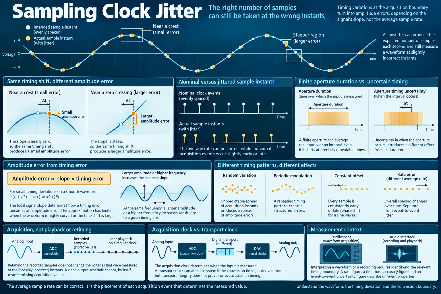
A converter can produce the expected number of samples each second and still measure a waveform at slightly incorrect instants. Its average rate describes how frequently measurements arrive over an interval. It says less about the placement of each individual measurement within that interval. Those placements matter whenever the voltage changes between nearby instants.

Sampling clock jitter describes variation in the timing of acquisition events relative to their intended positions. A sample collected a little early or late belongs to a different point on the incoming waveform. If the recording treats it as the value at the intended instant, the timing deviation appears as an error in the recorded amplitude. The same timing deviation can produce a tiny error on a slowly changing part of a waveform and a larger error on a steep part.

This explanation concerns acquisition: the moment an analog signal becomes a measured value. It does not require a wrongly labeled sample rate, a change in playback speed, or progressive drift between separate recordings. A clock can have the correct average rate while individual acquisition events fluctuate around their expected positions.

Signal slope determines how a timing error becomes an amplitude error

Consider a smooth sine wave and two intended sample positions. One sits at a positive maximum. The other sits at a crossing through zero. Move both sample positions slightly later by the same amount. The sample near the maximum changes relatively little because the curve is nearly horizontal there. The sample near the crossing changes more because the curve rises or falls rapidly.

The relevant quantity is the local signal slope: the rate at which the incoming value changes with time. A horizontal displacement along a steep curve produces a substantial vertical displacement. A similar horizontal displacement along a flatter curve produces less vertical change. The converter does not need to change its voltage sensitivity for this effect to occur. It has measured a different point on the input.

This also explains why amplitude and frequency both matter for a sine wave. At the same frequency, increasing the amplitude stretches the waveform vertically and increases its steepest slope. At the same amplitude, increasing the frequency packs the same rise and fall into less time. Both changes can increase sensitivity to a given amount of timing uncertainty.

A related example appears in the guide on amplifier slew rate. That topic asks why an amplifier can handle a small signal yet struggle with a larger signal at the same frequency. Its treatment of signal slope helps identify how amplitude and frequency set the rate of voltage change. The physical limitation differs: an amplifier may struggle to produce the required rate of change, while a sampler with uncertain timing may measure a changing input at the wrong position.

The small-error approximation and its limits

Let x(t) represent the true input value at an intended acquisition time t. Suppose the actual sample occurs at t + δt. The measured value is x(t + δt), so its error relative to the intended value is x(t + δt) − x(t). For a sufficiently small timing deviation on a smooth waveform, a local straight-line approximation gives:

Amplitude error ≈ local rate of change × timing deviation.

In symbols, this is x(t + δt) − x(t) ≈ x′(t)δt. The derivative x′(t) is the local signal slope. The units make the relationship useful: a slope expressed in volts per second, multiplied by a timing deviation expressed in seconds, gives an amplitude error expressed in volts.

A purely illustrative calculation shows the conversion. If the local slope were one volt per microsecond, a timing deviation of one nanosecond would correspond to approximately one millivolt of amplitude error. These chosen values demonstrate the arithmetic; they are not a measurement of a device or a claim about a recording system.

The approximation works when the waveform remains close to its tangent over the timing displacement. The curvature of the waveform determines how quickly that local straight-line description becomes inadequate. Near a sine-wave maximum, the first derivative is zero. The first-order formula therefore predicts zero error at the exact maximum, although a finite displacement still changes the measured value through higher-order terms.

A sharp transition needs more care. If a timing displacement carries the sample across a substantial part of an edge, a single local slope may represent the interval poorly. The same concern applies when the deviation is large relative to the time scale on which the waveform changes. Comparing the actual values x(t + δt) and x(t) remains valid; replacing their difference with one derivative times one displacement may cease to be accurate.

The approximation also assumes that timing displacement is the effect under discussion. A practical converter may have other errors at the same time. Separating those contributions requires suitable evidence. The equation by itself does not establish that timing uncertainty caused a particular feature in a captured waveform.

Aperture jitter belongs to the acquisition boundary

A converter has a sampling process inside its hardware as well as a clock signal reaching that hardware. Variation in the effective acquisition instant can arise along that path. The term aperture jitter is used for uncertainty in the converter’s effective sampling timing. A useful analysis identifies which timing contribution a specification or measurement describes, instead of treating every clock-related number as interchangeable.

Timing uncertainty also needs to be distinguished from the duration over which a measurement is formed. A finite sampling aperture can average the input over an interval. Even if that interval starts at precisely repeatable times, averaging may change the relationship between the output samples and the instantaneous input. Uncertainty in when the interval occurs introduces a different effect.

The related sampling-aperture guide explains how a measurement can represent a time average. Its discussion provides useful context for aperture jitter: the width of a measurement interval and uncertainty in its placement need separate descriptions. A wider interval does not automatically imply less stable timing, and repeatable interval placement does not make a finite average identical to an instantaneous sample.

For the timing-to-amplitude mechanism, the important event is the effective measurement of the input. Moving an earlier digital edge matters to this article only insofar as it changes that event. A clock specification needs a stated measurement point and operating conditions before it can support a conclusion about acquisition error.

Random variation, periodic modulation, fixed delay and rate error

Several timing patterns can leave the average sample rate looking reasonable. Their effects differ because the deviations have different structures.

Random timing variation gives acquisition events an unpredictable spread around their intended positions. Where the input changes quickly, that spread translates into a spread of amplitude errors. The resulting behavior depends on both the timing statistics and the waveform being sampled. A timing figure alone cannot describe every input-dependent consequence.

Periodic timing modulation moves acquisition positions according to a repeating pattern. For example, imagine the positions alternately advancing and retreating in a regular sequence while their long-term average spacing remains unchanged. The amplitude errors then follow the repeating timing pattern and the changing slope of the input. Structured timing modulation can create structured errors instead of an uncorrelated spread.

A constant offset shifts every acquisition event by the same amount. Relative to an external time reference, every recorded value belongs to a consistently displaced instant. For a sine wave, this amounts to a consistent phase displacement. The offset matters when absolute timing or alignment matters, but it does not create the same varying error pattern as event-to-event timing uncertainty.

An average-rate error changes the overall spacing of acquisition events. Its accumulated timing difference grows relative to an ideal reference. That is a separate quantity from fluctuation around a correctly spaced schedule. A clock can have a rate error, jitter, or both; an analysis should state which one its evidence supports.

These distinctions explain why counting samples over a long interval cannot fully characterize sampling clock jitter. Equal totals can arise from different arrangements of individual positions. A count describes the interval’s aggregate rate, while the acquisition error depends on the positions at which the input was actually measured.

Why retiming the recorded samples does not automatically repair them

After conversion, a recorded sample is a stored number. Suppose that number was acquired late, when the input had already moved to a different value. Delivering the stored number on a newly regular digital schedule changes when the number is presented. It does not change the voltage that was measured earlier.

This is why a downstream clock that schedules perfectly even output events cannot, by timing regularity alone, restore the missing acquisition values. The output may be orderly while carrying numbers associated with displaced input instants. The information needed for a correction goes beyond the existence of a clean later schedule.

If actual acquisition times were known, and the signal satisfied suitable assumptions, a reconstruction method might use those times to estimate values on a desired time grid. That possibility requires additional timing information and a defensible signal model. Ordinary retiming of an existing stream does not automatically supply either.

The limitation becomes clearer by imagining two possible inputs. They can agree at the actual measurement instants yet differ at the intended instants. The recorded values alone would then be insufficient to choose the correct intended values without further assumptions. A later clock cannot decide which input occurred merely by presenting the same numbers more regularly.

The timing problem must therefore be located along the chain. Acquisition uncertainty concerns how values were obtained. Output timing concerns when existing values are used. A particular system may connect those stages closely, but the connection needs to be established for that system rather than assumed from the presence of a digital clock.

An acquisition clock and a buffered transport clock have different jobs

A digital transport carries sample values between parts of a system. A buffered converter can receive those values, hold them in memory, and use a local clock to determine when it consumes or converts them. Within the operating limits of that design, variation in arrival times may change buffer occupancy while leaving the local conversion schedule unchanged.

For an analog-to-digital converter, its acquisition clock determines when the analog input is measured. For a digital-to-analog converter, the relevant local timing determines when stored values contribute to the analog output. The timing-to-amplitude reasoning applies at the conversion boundary where timing positions affect the resulting signal.

A transport clock can still matter if the conversion timing is derived from it or if disturbances in the transport path affect the local timing. Buffering is a design feature to investigate, not evidence that every possible timing influence has been removed. The key question is how the actual converter establishes its effective acquisition or conversion instants.

This distinction prevents a common analytical shortcut: treating variation in digital packet or sample arrival times as a direct measurement of analog acquisition uncertainty. The two observations may be related in a particular architecture. Establishing that relationship requires knowledge of the buffering and clocking arrangement.

It also prevents the opposite shortcut. A buffer’s presence does not prove the values were originally acquired at correct instants. A recording made with uncertain acquisition timing can be transported and buffered successfully while retaining the original measured errors. Transport integrity and acquisition accuracy answer different questions.

Using acquisition equipment without attributing unmeasured performance

The ZT-703S handheld oscilloscope, multimeter and signal generator listing describes a device that combines those three functions, including dual-channel waveform acquisition and waveform storage or export. The displayed waveform comes from measurements made at particular instants, so interpreting its trace requires distinguishing acquisition timing from the instrument’s aggregate rate figures. Its listed time-base accuracy and sampling rate describe specified aspects of operation, but those figures alone do not establish the effective timing uncertainty of a particular measurement.

The Focusrite Scarlett 4i4 fourth-generation recording bundle listing describes a four-input USB-C interface with four balanced outputs, supplied with recording accessories and monitors. A recording interface turns analog inputs into sample values and uses stored values to produce outputs, placing conversion timing at both ends of that path. The listing does not, by itself, establish a measured jitter result or an audible improvement attributable to a clock. Those conclusions would require evidence for the specific operating conditions and comparison.

For either kind of equipment, identifying the relevant timing boundary comes before interpreting a clock-related specification. A rate figure, a time-base accuracy figure and an event-to-event uncertainty figure describe different properties. Assigning one to the job of another can lead to a confident conclusion that the available measurement does not support.

What a useful explanation of a timing problem should establish

Start with the waveform being measured and the intended acquisition positions. Determine how rapidly the input changes near those positions. The comparison between a waveform maximum and a steep crossing gives a practical check on whether the explanation accounts for input-dependent sensitivity.

Then describe the timing deviation. State whether it is random, periodic, constant, or an accumulating rate difference. Use the small-error approximation only over an interval where the local straight-line description is reasonable. Where it is unsuitable, compare the waveform values at the actual and intended instants directly.

Finally, separate acquisition from later delivery. Identify whether the observed timing belongs to an analog sampling boundary, a digital transport, or the local schedule of a buffered converter. This makes it possible to explain why a correct average sample rate can coexist with inaccurate acquired amplitudes, and why regularizing a later schedule may leave those amplitudes unchanged.

When evaluating an explanation, look for the actual measurement position, the input’s rate of change there, and the timing deviation that is being claimed. Those quantities support a calculation of acquisition error. A rate label alone leaves the event positions unspecified; an output clock alone leaves the previously acquired values unspecified.