Amplifier slew rate: why bandwidth does not guarantee clean large signals

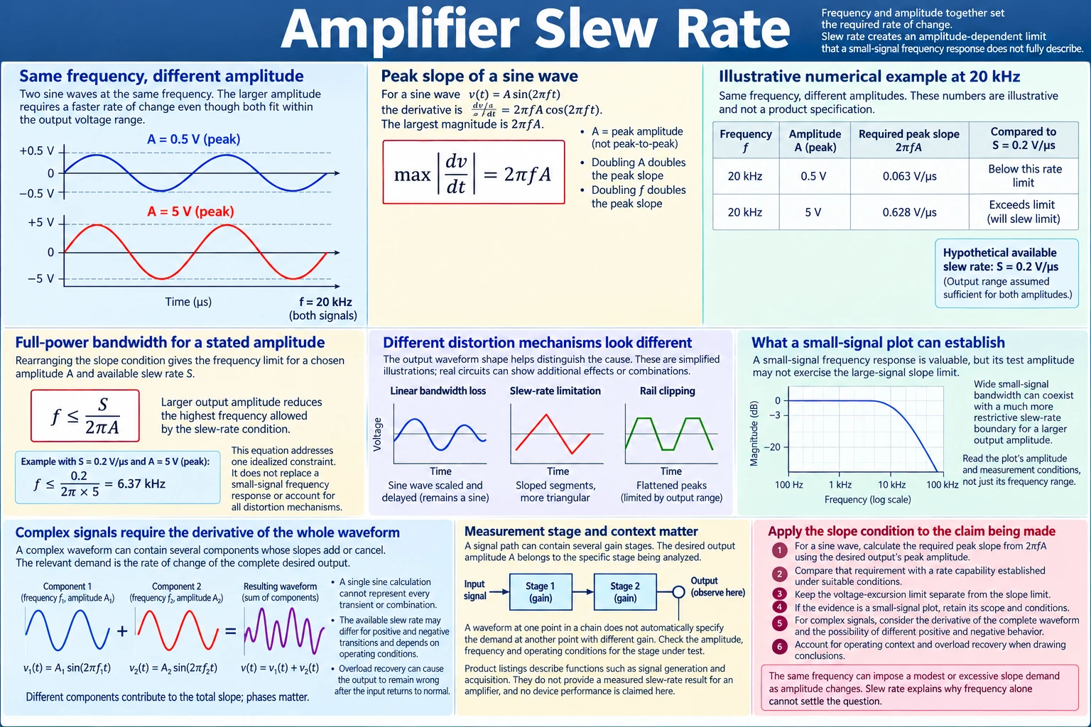
An amplifier can reproduce a small sine wave cleanly at a frequency where a larger sine wave becomes distorted. Both signals can fit within the amplifier’s available output-voltage range. Their different behavior can arise because the larger wave requires the output voltage to change faster.

Amplifier slew rate describes a limit on that rate of voltage change. It creates an amplitude-dependent constraint that a small-signal frequency-response plot does not fully describe. Frequency matters, but the desired output amplitude matters with it.

A local linear response, a limit on changing voltage and a limit on voltage itself can all affect the same circuit. Each describes a different requirement imposed by the desired output.

Keep the frequency fixed and change the amplitude

Imagine a sine wave that completes the same rise and fall in every cycle. Make its amplitude ten times larger while keeping the frequency unchanged. The period stays the same, but the output must now traverse ten times the voltage distance over the corresponding parts of that period.

Near a maximum or minimum, the sine changes relatively slowly. Near a crossing through its midpoint, it changes most rapidly. Enlarging the sine stretches the required rate of change at every corresponding position, including those steep crossings.

A linear amplifier would scale the waveform according to its frequency response while preserving the sinusoidal shape in steady state. If its response at that frequency were unchanged with amplitude, the larger input would produce a proportionally larger output. A slope constraint can prevent that proportional relationship even before the output reaches a voltage limit.

Compare the required output slope with the available slope under the relevant operating conditions. A frequency that is comfortably within a small-signal response specification can still demand too much rate of change when the desired amplitude is large.

Deriving the peak slope of a sine wave

Write the desired output as A sin(2πft), where A is its peak voltage amplitude and f is its frequency. Differentiating with respect to time gives 2πfA cos(2πft). The largest absolute value of that derivative is therefore 2πfA.

The result has a straightforward interpretation. Doubling the desired amplitude doubles the greatest required slope. Doubling the frequency also doubles it. Increasing both by the same factor multiplies their effects. The available amplifier slew rate must be considered against the combination rather than against frequency alone.

A denotes the peak amplitude of the desired output, not its peak-to-peak excursion. A sine that travels from −A to +A has a peak-to-peak swing of 2A. Mixing those definitions would change the calculated slope requirement by a factor of two.

Consider an explicitly hypothetical example. At 20 kilohertz, a desired output amplitude of 0.5 volts has a peak slope of approximately 0.063 volts per microsecond. Increasing the desired amplitude to 5 volts at the same frequency raises the requirement to approximately 0.628 volts per microsecond.

Now imagine a device with an available slope of 0.2 volts per microsecond and an output range sufficient for either desired amplitude. The smaller sine’s slope requirement falls below the stated rate limit. The larger sine’s requirement exceeds it. The calculation explains how an amplitude-dependent problem can arise without the desired peaks touching the voltage boundary.

These numbers illustrate the equation. They are not specifications or measurements for the products linked below. An actual device would need a suitable slew-rate value and a clear statement of its conditions before the calculation could support a conclusion about its operation.

Full-power bandwidth requires a stated amplitude

Rearranging the sine-wave slope condition gives a frequency boundary for a chosen amplitude. If S denotes the available rate of voltage change, the idealized condition is 2πfA ≤ S, or f ≤ S/(2πA).

This is the basis for discussing full-power bandwidth in relation to a specified large output amplitude. Reducing that amplitude raises the frequency allowed by this particular slope condition. A frequency range quoted without its amplitude leaves an important part of the requirement unspecified.

Using the hypothetical 0.2-volts-per-microsecond rate and a 5-volt peak sine, the boundary from this equation is about 6.37 kilohertz. That does not mean a real amplifier meeting those nominal quantities would remain undistorted at every frequency below the calculated boundary. The equation addresses one idealized constraint, and a practical performance criterion can require additional margin.

It also does not replace a small-signal frequency response. A circuit can encounter linear amplitude loss or phase shift independently of its large-signal rate capability. Satisfying one condition does not establish that the other response is flat, or that the complete output has met a chosen accuracy requirement.

The sampling-aperture guide derives how averaging over a finite measurement interval changes a sinusoid before its values are reported. That comparison helps interpret full-power bandwidth: the aperture model’s attenuation depends on frequency and window duration, whereas the amplifier’s sine-wave slope condition also depends on the desired output amplitude. Both analyses require a stated model, but their equations describe different operations along a signal path.

Linear bandwidth loss, large-signal distortion and rail clipping

In a linear bandwidth-limited response, a steady sine wave can remain a sine wave while its amplitude is reduced and its phase changes. The frequency-response relationship predicts those changes within the conditions where the circuit remains linear.

A slew-limited response instead encounters a bound on how rapidly the output can move. Where the requested slope exceeds that bound, the output cannot follow the desired trajectory. A simplified hard slope limit can produce segments with nearly constant rates of change. With sufficiently demanding periodic signals, the output can become more triangular than sinusoidal, although the details of a real response depend on the circuit.

Rail clipping limits the output excursion. If a desired voltage lies beyond the available range, the output cannot reach it. A simplified voltage limiter produces flattened extrema. This limit concerns how far the output can travel, while slew limitation concerns how rapidly it can travel within its range.

These simplified shapes are useful for separating mechanisms, not for identifying every real circuit from the appearance of one trace. A circuit can encounter multiple constraints during the same waveform. Its nonlinear behavior and recovery can also change the observed shape.

The term large-signal distortion therefore needs a mechanism attached to it. If a high-amplitude sine has become distorted, a frequency response measured at a much smaller amplitude does not establish whether the cause was a slope limit, an excursion limit, or another behavior that appeared under the larger demand.

In the slope example, the desired 5-volt peak remains within the imagined available voltage range, yet the required rate exceeds the imagined slope capability. That is the distinction the example was built to isolate. It does not require an earlier clipped recording or a claim about a particular amplifier’s audible performance.

What a small-signal plot can establish

A small-signal test examines behavior around an operating condition where the applied disturbance is small enough for the local response to be treated as approximately linear. Its frequency-response plot is valuable evidence about that test. It does not automatically describe what happens when the output must cover a much larger voltage excursion in the same time.

If the test amplitude makes the peak slope demand comfortably smaller than the available rate, the measurement may never exercise the large-signal constraint. A wide small-signal response can therefore coexist with a much more restrictive slope boundary for a larger desired output.

Reading the plot requires its amplitude and measurement conditions, not just its horizontal frequency range. A result produced with a small disturbance cannot silently be relabeled as evidence of large-output capability. The extrapolation needs a basis in the device’s operation or an appropriate measurement.

The distinction applies even when the chosen frequency looks unremarkable on the plot. The product fA determines the sine’s peak slope. A large A can make that product demanding at a frequency that a small-amplitude test handles easily.

For a comparison between devices, keep the relevant amplitude definition and conditions consistent. Otherwise two figures may appear to describe the same capability while referring to different demands. A local frequency response and a large-signal rate limit should each retain the question they actually answer.

Complex signals require more than one sine-wave calculation

The sine calculation is useful because its maximum derivative has a simple expression. A complex waveform can contain several components whose slopes add or partly cancel at particular instants. Considering each component independently does not always give the maximum slope of their combined time waveform.

The relevant demand is the rate of change of the complete desired output. Its largest value depends on the amplitudes, phases and temporal alignment of the components. A single chosen sine frequency cannot represent every transient or combination present in a program signal.

The available rate may also need a more complete description than one nominal number. Positive and negative transitions can have different behavior, and the stated operating conditions matter. A calculation based on one value should acknowledge the conditions and direction it represents.

The sampling-clock-jitter guide shows how waveform slope converts uncertainty in acquisition time into an error in the measured amplitude. Its derivation offers a useful comparison when examining large-signal distortion: both explanations depend on how rapidly the waveform changes, but the jitter model moves the measurement instant while the slew model limits the amplifier’s ability to produce the requested trajectory. Distinguishing the mechanisms prevents a slope-dependent measurement error from being assigned automatically to an amplifier limit.

That distinction limits what can be inferred from the sine inequality. The inequality can reveal that a particular desired slope exceeds a stated capability. Meeting it does not independently establish the absence of every nonlinear effect, a specified distortion level for complex material, or an audible result.

Using listed equipment without inventing an amplifier result

The waveform-generator and acquisition functions listed for the ZT-703S handheld oscilloscope, multimeter and generator make signal generation and observation relevant uses of that instrument. The slope question concerns the actual waveform demanded from a circuit and the waveform observed under the chosen conditions. Its listing does not supply a measured slew-rate result for an amplifier connected to it, and the hypothetical sine calculation here should not be attributed to the instrument.

The Focusrite Scarlett 4i4 fourth-generation recording bundle includes an audio interface and monitoring equipment in its described contents. A recording and monitoring setup can contain several signal-gain stages, so the distinction between output amplitude, frequency response and rate of change is relevant to understanding a path. The product description provides no basis here for assigning the hypothetical slope limit to a particular stage or making a claim about its audible performance.

For an actual evaluation, the desired output amplitude and frequency must be associated with the stage being examined. A waveform at one point in a chain does not automatically specify the demand at another point with different gain. The quantity A in the slope calculation belongs to the desired output of the stage under analysis.

Apply the slope condition to the claim being made

For a sine wave, calculate the required peak slope from 2πfA using the desired output’s peak amplitude. Compare that requirement with a rate capability established under suitable conditions. Keep the voltage-excursion limit separate so that slope limitation is not mistaken for reaching a rail.

If the available evidence is a small-signal frequency plot, retain its scope. It describes the response to its stated small disturbance. Establishing large-output behavior requires information that addresses the larger voltage distance being traversed in the same cycle.

Amplifier slew rate explains why frequency alone cannot settle the original question. The same frequency can impose a modest or excessive slope demand as amplitude changes. The sine calculation gives a specific boundary to examine, while the complete waveform, operating conditions and earlier time history determine how far that boundary can support a practical conclusion.