Sampling aperture: why a sample can be a time average

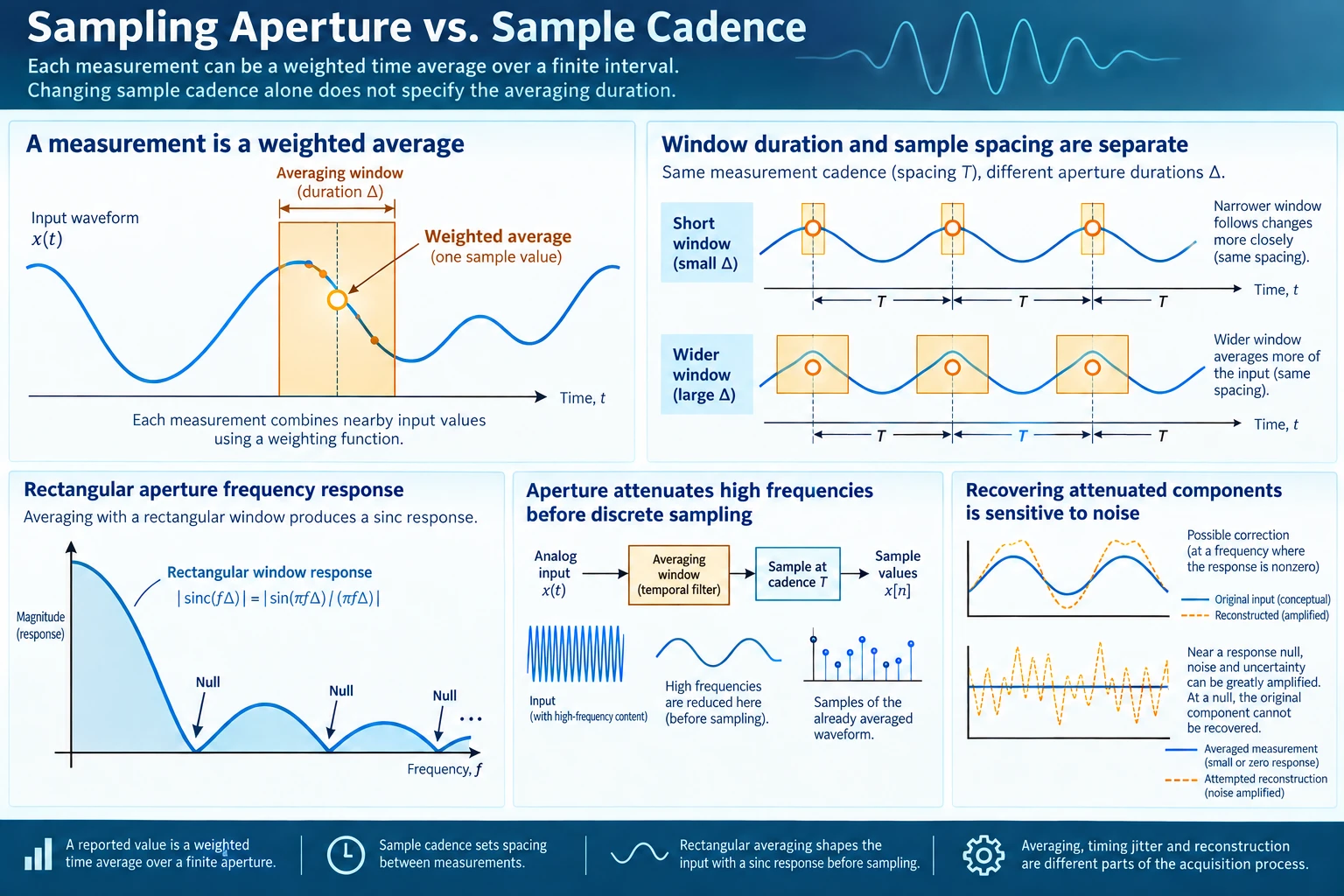
A measurement delivered every millisecond does not necessarily describe the input at one isolated instant. It may summarize what happened across a finite interval. Producing more of those summaries each second changes their spacing, while the width of the interval used for each summary may remain unchanged.

A finite sampling aperture describes the temporal extent of an acquisition measurement. When the measurement averages the input across that extent, it filters the input before the resulting values are treated as samples. Rapid changes within the interval can partly cancel, leaving a smaller measured variation even when the output values arrive at a high rate.

The distinction is between the timing of reported values and the temporal operation that produces each value. A high output cadence supplies many measurements of the filtered input. It does not automatically make that input identical to the original waveform.

Writing a measurement as a weighted average

Let x(t) represent a continuously changing input. An ideal instantaneous measurement at time t would return x(t). An interval measurement can instead be written as an integral of nearby input values multiplied by a weighting function. In words, it adds contributions from different instants, with the weighting function determining how much each instant contributes.

Normalizing the weighting so that its total weight is one gives a useful average: a constant input remains unchanged. That condition establishes the response to a steady value. It does not imply that every time-varying input will retain its amplitude or shape.

A simple model uses a rectangular weighting function. Every instant within a window of duration Δ receives equal weight, and instants outside the window receive none. A measurement centered on t is then the integral of x over the interval from t − Δ/2 to t + Δ/2, divided by Δ.

Other weighting shapes are possible. The rectangle is useful because its consequences can be derived explicitly. An actual device would need evidence about its acquisition process before this particular shape could be assigned to it. Calling a measurement an average does not establish that all contributing instants receive exactly equal weight.

Mathematically, this is a temporal convolution followed by evaluation at the reported sample positions. The convolution determines which aspects of the continuous input survive into the averaged signal. The sample positions determine where that already modified signal is recorded.

Integration time and sample spacing are separate quantities

Suppose a system reports values at positions separated by T seconds. Its output rate is 1/T. Suppose each reported value averages a window Δ seconds wide. The ratio between Δ and T describes whether the windows are separated, touch, or overlap, but neither quantity determines the other in the mathematical model.

If Δ is smaller than T, each average can cover only part of the interval between reported values. If Δ equals T, successive rectangular windows can touch without overlapping. If Δ is larger than T, adjacent averages include some of the same input history. These arrangements describe the observations being formed; they do not change the definition of their output cadence.

The integration time can therefore stay fixed while the reporting rate increases. The system may deliver more densely spaced evaluations of the same averaged signal. Overlapping windows can make those observations share input information, so the additional reported values should not automatically be interpreted as independent measurements of untouched instantaneous inputs.

The sampling-clock-jitter guide explains how uncertain acquisition positions become amplitude errors through the input’s local slope. Its comparison of a finite measurement interval with uncertain interval placement helps keep integration time separate from timing stability. An average formed over a known interval can still occur too early or too late; a repeatably placed interval can still attenuate a changing input.

For the acquisition problem, the important question is what waveform has been averaged before the values are reported. Raising the number of reports per second addresses the spacing of observations. To address attenuation introduced by their construction, the analysis must also consider the weighting window.

Deriving the rectangular window’s aperture response

Take a sine or cosine input with frequency f and average it over a centered rectangular window of duration Δ. Integrating the sinusoid over that interval gives the same sinusoid at the window center multiplied by a frequency-dependent factor:

Amplitude factor = sin(πfΔ) / (πfΔ).

At zero frequency, the ratio has a limiting value of one, consistent with the normalization that preserves a constant input. At other frequencies, the factor describes how the rectangular average changes the sinusoid. Its magnitude gives the amplitude ratio, and its sign indicates whether the resulting sinusoid is reversed relative to the centered reference.

The product fΔ sets the behavior. It counts how much oscillation occurs within one averaging interval. When the input varies slowly compared with the window duration, neighboring values have similar signs and sizes, so their average remains close to the value at the center. As more variation fits into the interval, cancellation becomes stronger.

For a purely mathematical example, let the averaging window span half a period of the sinusoid. Then fΔ is one half, and the amplitude factor is 2/π, approximately 0.637. The measured sinusoidal variation is therefore about sixty-four percent of the original amplitude in this model. Reporting these averages at more positions does not change that factor if the window width stays fixed.

If the window spans a complete period, fΔ is one. The positive and negative contributions cancel exactly in the ideal rectangular model, and the factor is zero. A sufficiently high reporting rate can then produce many zero-valued averages of a sinusoid that was present at the input.

This calculation specifies an ideal weighting function and input. It is not a performance measurement of an instrument. A differently shaped window has a different frequency response, and an actual acquisition path may introduce other effects in addition to averaging.

Attenuation can occur before any spectral folding

The loss in these examples comes from averaging within each window. It can exist even when the output sample spacing is sufficient for representing the averaged waveform without ambiguity. The input is modified before the sequence is formed.

This ordering separates aperture-related attenuation from insufficient output sampling rate. In the first case, the temporal weighting changes the waveform being observed. In the second, the spacing of observations can make different waveform variations produce an ambiguous sequence. Both processes may occur in a system, but increasing the reporting rate addresses only the latter spacing question unless the acquisition window changes as well.

Consider again the half-period window, with its amplitude factor of about 0.637. Place the output sample positions sufficiently close together to represent that averaged sinusoid. The samples can describe the reduced-amplitude sinusoid accurately while still differing from instantaneous samples of the original input.

A reconstruction of those reported values can consequently be faithful to what was measured and still have a smaller variation than the input originally had. Reconstruction begins from the averaged observations. It cannot assume that each stored value came from an ideal instantaneous acquisition when the measurement model says otherwise.

The aperture response belongs in the acquisition path’s overall description. It determines how the window affects variations before later sampling and reconstruction are analyzed. Ignoring that stage can turn a correctly reproduced averaged waveform into an apparently unexplained amplitude discrepancy.

Window position affects phase as well as amplitude

The centered-window derivation uses the middle of each interval as its time reference. If a reporting convention associates the same interval with its start or end instead, the averaged sinusoid is being labeled with a displaced time reference. The window’s location then needs to be included in the phase relationship.

For example, an average over a fixed interval ending at the reporting time summarizes values from the preceding interval. Comparing it directly with an instantaneous value at that reporting time hides the difference between the interval’s center and its label. A consistent model states both the interval width and the position to which the result is assigned.

This phase consideration is deterministic in the stated window model. The interval can occur at precisely repeatable positions. Uncertainty in when a measurement occurs would require a separate timing description; the attenuation derived here already exists without such uncertainty.

The amplifier-slew-rate guide derives the maximum slope required by a sine wave and explains why a larger amplitude can exceed an amplifier’s rate limit at an otherwise manageable frequency. Comparing that mechanism with the aperture response helps distinguish two ways a signal path can alter a waveform. The rectangular average has a linear, frequency-dependent response at any amplitude in this model; a slew limit depends on the rate of change demanded by the actual output waveform.

When interpreting a captured pulse, a ramp or a sinusoid, identify the time reference of the measurement before comparing it with a point on the input. Otherwise an interval measurement can be judged against an instantaneous reference that it was never intended to reproduce.

Why inversion becomes fragile near a response null

If the averaging model is known, one might attempt to compensate for its attenuation. For a sinusoid at a frequency where the response factor is nonzero, the ideal calculation would divide the observed amplitude by that factor. This describes a possible mathematical correction under the stated model.

A small response factor makes that division sensitive to imperfections. Measurement noise, numerical error and uncertainty in the window model can be magnified by the same correction. The closer the factor is to zero, the greater the amplification required to recover a specified input amplitude from a small observed result.

At an exact null of the ideal rectangular response, the average provides no amplitude information about that sinusoidal component. Different amplitudes at the nulled frequency produce the same zero contribution to the averaged observations. More densely sampling those observations cannot distinguish the amplitudes that the averaging operation has canceled.

This is a loss of information within the model. Choosing a later interpolation method does not supply the missing contribution. Recovery would require additional observations or assumptions that distinguish the possible inputs, rather than treating the null as a small attenuation that can always be reversed safely.

A practical compensation method must also account for how well the model describes the actual weighting window. Correcting an assumed rectangular response can introduce errors if the real acquisition process has another shape. The existence of a neat formula does not establish the required identification of a device’s acquisition behavior.

Acquisition equipment and the limits of a listing

The ZT-703S handheld acquisition instrument combines an oscilloscope with multimeter and waveform-generator functions in its listing. Its acquisition and waveform-storage features make it relevant to the distinction between a reported measurement and an instantaneous input value. The listed sample rate does not, by itself, specify a rectangular weighting window or establish the width of an effective acquisition interval. Those details would need evidence for the actual measurement process.

The recording setup described by the Focusrite Scarlett 4i4 fourth-generation interface bundle includes a four-input USB-C audio interface and recording accessories. Its analog-input role provides another context for asking what an acquired value represents before it enters a digital recording. The bundle description establishes its stated functions and contents, but it does not justify assigning the rectangular averaging model in this article to that interface or inferring a device-specific amplitude correction.

Interpreting a rapidly reported average

A useful measurement description states the output spacing, the interval width, the weighting shape and the time assigned to each result. Together, those quantities describe how the input contributes to the reported values. The output rate alone leaves the interval operation unspecified.

For a rectangular sampling aperture, the factor sin(πfΔ)/(πfΔ) shows the consequences directly. A half-period interval reduces the sinusoidal amplitude in the ideal model, while a full-period interval cancels that component. Both effects can occur before any ambiguity caused by output sample spacing.

If compensation is being considered, identify where the response remains well away from zero and how confidently the window is known. Near a null, inversion may amplify uncertainties severely; at the null, the original observations do not retain the canceled component’s amplitude. Higher reporting cadence gives more evaluations of the averaged signal, but restoring an instantaneous signal requires information that survived the averaging operation.