Intersample peaks: why safe digital samples can reconstruct above full scale

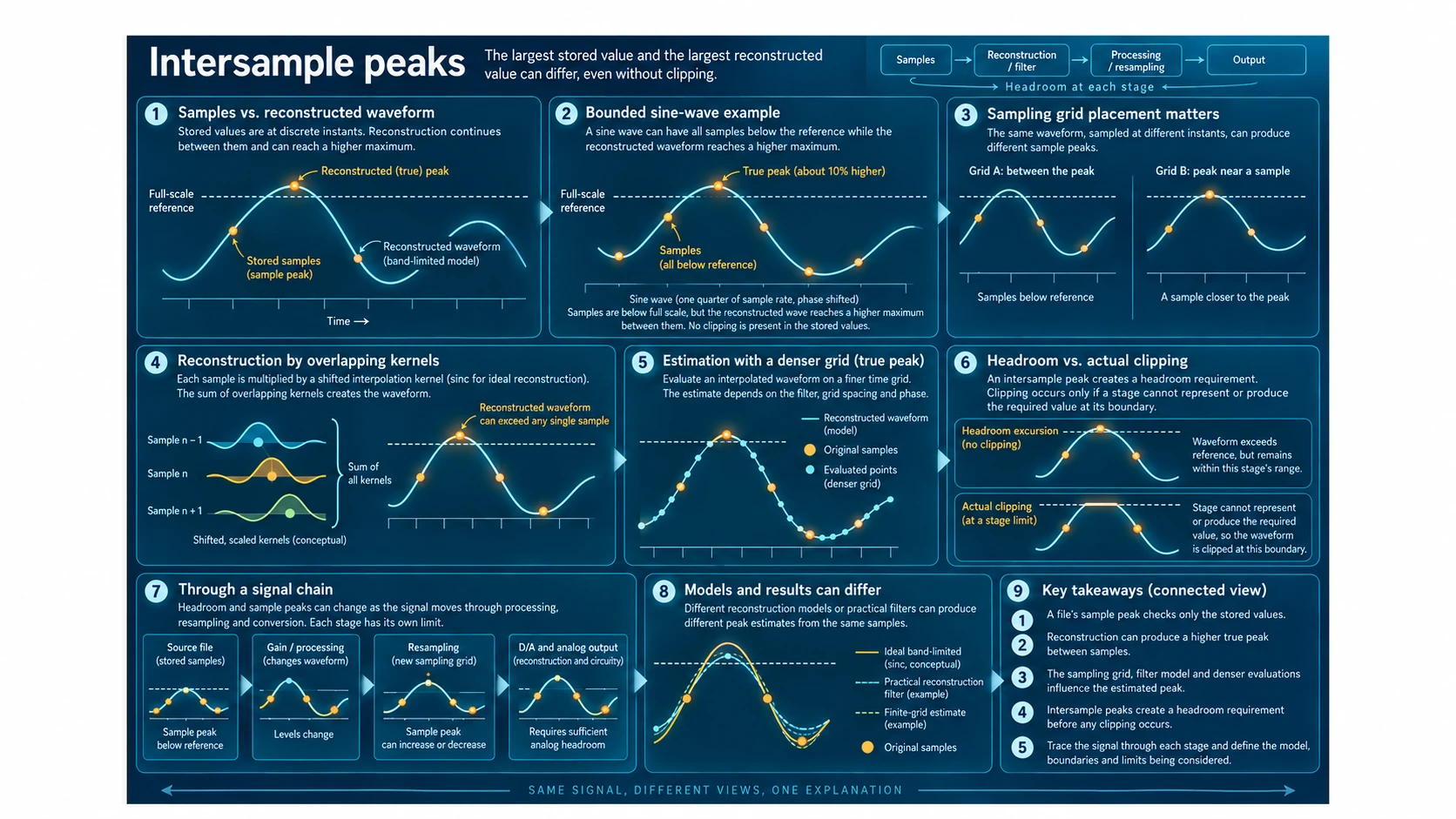
A digital recording stores values at a sequence of instants. A playback system produces a waveform that continues through the intervals between those instants. The largest stored value and the largest value of that reconstructed waveform can therefore differ, even when the recording has never been clipped.

Intersample peaks are maxima that occur between the original sample positions. They explain how a file whose stored values stay below a chosen full-scale reference can require more headroom during reconstruction. A limit applied only to the stored numbers does not inspect every point the reconstructed signal can reach.

The distinction matters before overload occurs. A waveform may contain an intervening maximum without having suffered clipping anywhere in the chain. Clipping enters the explanation only when a particular stage cannot represent or produce the values required at its own boundary.

Sample peak checks the stored values

For a discrete sequence, finding the largest absolute sample value is straightforward in principle: inspect the numbers and retain the greatest magnitude. This sample peak measurement describes what is present at the sample positions. It does not require an estimate of the intervening waveform.

A reconstructed maximum asks a different question. It concerns a waveform generated from the sequence under a particular reconstruction model. That waveform has values at the original positions and at the positions between them. The original sample values constrain its behavior, but they do not constitute a list of every value it will take.

Connecting adjacent values with straight lines would keep each segment between its endpoint values. Such a drawing can make a sequence look safely bounded by its largest stored value. A band-limited reconstruction uses a different shape. Treating a straight-line display as a proof about that reconstruction substitutes one model for another.

The term full scale also needs a reference. In the example below, a magnitude of one represents the chosen normalized level. This avoids confusing the mathematical demonstration with the precise largest integer code in a specific file format or the voltage available at a particular analog output. Those implementation limits must be established separately.

A bounded example with a larger intervening maximum

Imagine a sine wave with a frequency equal to one quarter of the sample rate. Its period spans four sampling intervals. Shift its phase so that the first two samples sit on either side of the positive maximum, and give the continuous wave an amplitude of 1.10 relative to the normalized reference of one.

Writing sample position as n, the ideal sequence is 1.10 × sin(πn/2 + π/4). At the integer positions, the values repeat approximately 0.778, 0.778, −0.778, −0.778. Every stored value has a magnitude below one. The samples are consistent with an unclipped sequence relative to that reference.

The positive maximum occurs halfway between the first two sample positions. There the continuous sine wave reaches 1.10. The corresponding negative maximum also falls between positions and reaches −1.10. The maximum reconstructed magnitude is therefore ten percent above the chosen reference, even though the stored magnitudes are about twenty-two percent below it.

This is a mathematical example, not a test result for equipment or a recommendation about how much headroom a recording always needs. The waveform is a single sine below half the sample rate, and the stated reconstructed result assumes the ideal band-limited sine-wave reconstruction consistent with that sequence.

The example also shows why the gap is about sample placement. Move the sampling grid relative to the sine wave and some positions may land nearer its maxima. The measured sample peak can then change while the continuous sine still has the same amplitude. A maximum that falls between one grid’s positions may coincide with another grid’s positions.

There is no clipped plateau to repair in this example. The original sequence simply does not place samples at the waveform’s largest excursions. The reconstructed maximum follows from the waveform consistent with those samples and from the reconstruction being specified.

Overlapping interpolation kernels create the waveform

A useful description of reconstruction assigns an interpolation kernel to each sample. Each kernel has a shape centered on that sample’s position and is scaled by the sample value. The reconstructed signal is the sum of these shifted, scaled shapes.

For ideal band-limited interpolation, the kernel is a sinc function. At the original sample positions, its values allow the reconstructed waveform to pass through the sequence’s prescribed values. Between positions, several shifted kernels contribute to the same point. Their combined value can exceed the magnitude of any individual stored sample.

This sum does not behave like a rule that merely selects the larger neighboring sample. Nor is it generally a weighted average with exclusively nonnegative weights. The positive and negative parts of an interpolation kernel, together with the signs and positions of the samples, determine the result. Contributions from samples beyond the nearest pair can matter.

In the sine-wave example, the overlapping contributions reconstruct the continuous sine with amplitude 1.10. The repeated stored values of about 0.778 do not impose a ceiling of 0.778 on that sum. They specify the values at the original positions, where the reconstruction agrees with them.

A practical filter uses a finite implementation rather than an infinite ideal kernel. Its coefficients and operating conditions determine the waveform or estimate it produces. The ideal example establishes that the peak difference can exist; it does not guarantee that every implemented filter will produce precisely the same intervening values.

This is why a drawing of only the sample markers leaves part of the problem hidden. To assess intersample peaks, the analysis needs both the stored sequence and a defensible account of the waveform represented or produced between its points.

True peak depends on how reconstruction is modeled

A true peak estimate attempts to account for reconstructed maxima rather than inspecting only the original sample positions. A digital implementation often evaluates an interpolated representation on a denser time grid. That can reveal excursions that the original grid missed.

A finite oversampling calculation still needs an explicit model. Its interpolation filter, phase arrangement, boundary treatment and number of evaluated positions affect the estimate. Saying that a calculation uses more points describes its sampling density; it does not fully describe what curve those points are intended to approximate.

The estimated maximum can also depend on where the denser grid falls relative to the exact maximum. If the largest excursion lies between even those evaluated positions, the computed maximum may fall below the maximum of the modeled continuous waveform. A sufficiently appropriate grid can improve the approximation, but a finite set of evaluated values needs a stated accuracy claim rather than an assumption of exactness.

Different models may produce different estimates from the same source samples. An ideal band-limited reconstruction, a particular finite filter and a specific playback path need not have identical maxima. A meaningful comparison identifies the model used and the signal path whose headroom is being considered.

The guide on peak-hold response addresses another reason to distinguish a meter’s reported maximum from the input event being measured. A detector must acquire a short excursion and preserve its result until readout. That guide’s discussion of the input’s true peak concerns acquisition speed, retention and reset timing. Those mechanisms differ from digital interpolation, but they reinforce the need to define what a reported maximum actually represents.

A meter reading can be useful within its stated model and conditions. The reading alone does not certify every converter, analog output or later processing stage in a chain, and this explanation makes no product-specific meter-certification claim.

Stored clipping and reconstructed overload occur at different boundaries

Stored sample clipping happens when a sequence cannot represent the required values at its own discrete positions and the signal is limited there. A file may contain maximum-valued samples because of such limiting, although interpreting any particular file requires evidence about how it was produced.

Reconstructed-waveform overload can occur even when none of the stored values has reached that discrete limit. A downstream implementation may need internal values or an analog excursion larger than its available range. The sine-wave example provides the premise: all original values remain below one while the modeled waveform reaches 1.10.

Whether overload actually occurs depends on the stage. A calculation with enough internal range may represent values above the chosen normalized reference without clipping. A later output stage may have a different limit. The existence of an intervening maximum establishes a headroom requirement for a particular waveform, not proof that every path has violated that requirement.

Clipping is therefore a separate event to investigate. It is not an inevitable label for every instance of intersample peaks. It also does not follow that every excursion beyond a normalized reference is audible. Audible consequences would depend on what the actual path does to the signal and on the conditions of a comparison.

The subject here is the growth of a reconstructed peak before clipping. Restoring a recording that has already been clipped would require a different analysis. Reframing an existing sequence’s maximum does not reveal all of the information an earlier limiting operation may have removed.

Headroom changes as the signal moves through a chain

A gain change applied to a sequence scales its stored values. If the following reconstruction is linear and otherwise unchanged, it scales the reconstructed waveform as well. A gain decision based on one maximum therefore needs to account for which maximum is being controlled.

Resampling changes the positions at which the represented signal is evaluated. A new sequence can place a sample closer to an intervening maximum than the old sequence did. Its largest stored value may consequently differ, even when the stipulated conversion aims to preserve the same underlying signal.

The related guide on polyphase resampling explains how a rate converter reorganizes filtering work around the coefficient phases needed for its outputs. That offers useful context when tracing a sample peak through a rate change: the output grid and specified filter matter to the resulting values. Rearranging the calculation efficiently does not independently guarantee more headroom or change the stipulated filter’s result.

Another boundary appears when digital values produce an analog output. The converter’s reconstruction behavior and the output circuitry determine the analog waveform and available excursion. A digital reference level is not, by itself, a complete specification of that circuitry’s voltage margin.

Processing between these stages can complicate the trace further. If the processing changes the waveform, a previously measured maximum may no longer describe the result. Assessing the next stage then requires the values or waveform actually entering it, rather than a maximum retained from an earlier point in the chain.

A clear headroom account names each relevant boundary and its limit. It distinguishes the range of stored source values, the range used for intermediate calculations and the excursion produced at an output. Treating all of these as one interchangeable full-scale ceiling hides the reason an apparently safe source can challenge a later stage.

Equipment listings and the measurements they can support

The waveform storage and export functions listed for the ZT-703S handheld oscilloscope, multimeter and signal generator make the distinction between recorded points and a continuous input relevant to interpreting its captures. A displayed set of acquisition points is a description of what the instrument recorded. A trace or reported maximum needs an account of the acquisition method before it can support a conclusion about an intervening analog excursion. The listing alone does not certify a particular reconstructed-peak measurement.

An audio-interface output is one boundary at which stored values become an analog waveform. The Focusrite Scarlett 4i4 fourth-generation recording bundle includes a USB-C interface listed with four inputs and four balanced outputs, placing both recording and playback within the described setup. Establishing how a specific digital sequence behaves at an output would still require the relevant conversion conditions and measurements; neither the interface description nor the bundle contents supply a product-specific peak-meter certification.

These distinctions keep the role of equipment evidence clear. A listing establishes the described functions and supplied items. A mathematical reconstruction establishes the behavior of its specified model. A measurement establishes an observed result under its recorded conditions. Each supports a different part of the explanation.

Reading a peak result with the right question in mind

When a result seems contradictory, identify the signal representation being measured. A maximum over the original sample values can be correct while a maximum over a reconstructed waveform is larger. The two calculations inspect different sets of positions.

Use the bounded sine-wave example to check the distinction. Samples near 0.778 can belong to a continuous waveform with a maximum of 1.10. The gap follows from the grid’s phase relative to the waveform and from the stated reconstruction model, with no prior clipping required.

For a real signal path, specify the reconstruction or estimation method and trace subsequent gain, rate conversion and output limits. That provides a basis for deciding where margin is needed. A safe list of stored values supplies useful information about one boundary; it leaves the behavior between those positions and at later boundaries to be established.