How polyphase resampling computes only required rate-conversion samples

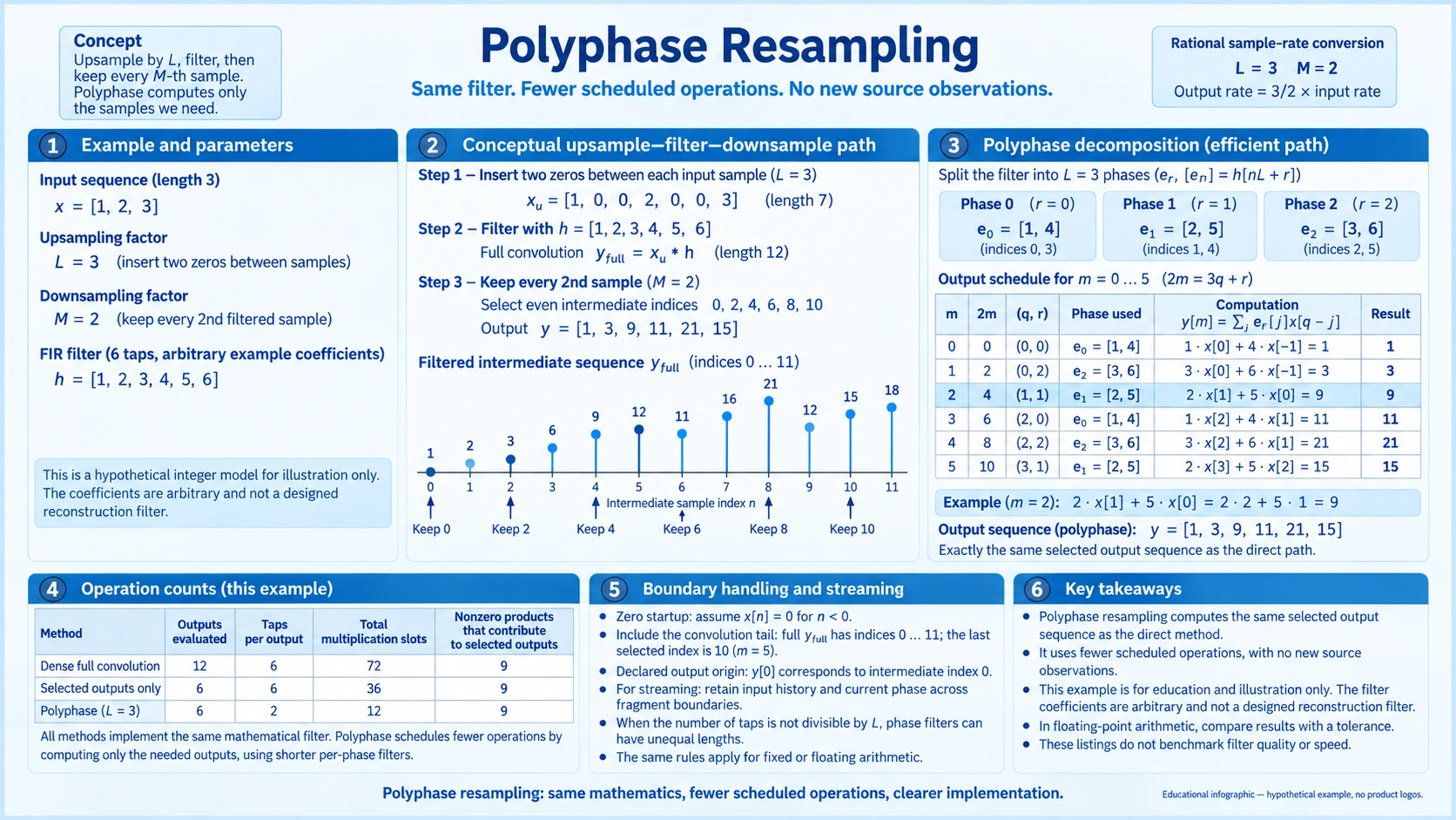
A rational rate converter can be described as inserting zeros, filtering the resulting sequence, and retaining selected outputs. That description defines the calculation but need not define the implementation. Most inserted values are zero, and many filtered samples will be discarded. Computing only the required terms can produce the same specified output.

polyphase resampling reorganizes that convolution according to the coefficient phase and input position needed by each output. The changed execution schedule avoids unnecessary arithmetic. The filter coefficients, output time origin, and boundary rules remain part of the model, so avoiding work does not independently improve filter response or create new measurements.

Specify rational sample rate conversion before scheduling it

Choose interpolation factor L = 3 and selection factor M = 2. The output rate is 3/2 times the input rate. Stipulate evenly spaced input samples x[n] at rate Fin, an intermediate grid at 3 Fin, and output m associated with intermediate index 2m. The output time is 2m/(3 Fin) relative to the declared zero origin.

Define the conceptual sequence u[k] as x[k/3] when k is a multiple of 3, and zero otherwise. Filter it with a causal FIR sequence h[j]. The intermediate result is v[k] = sum over j of h[j] u[k - j], and the required output is y[m] = v[2m]. These equations define the calculation without requiring an allocated zero-filled buffer.

Combining the steps gives y[m] = sum over n of x[n] h[2m - 3n], with coefficients outside the FIR support equal to zero. This equation exposes exactly which input values can contribute to a selected output. It also supplies the reference against which a reorganized implementation can be checked.

The sampling-aperture guide explains how averaging can attenuate an input before its samples are reported. This measurement history matters for rational sample rate conversion, which operates on the accepted samples. Reorganizing filtering cannot independently restore source detail that the measurement process did not retain.

Derive filter phase decomposition from the output equation

For each output, write 2m = 3q + r, where q is the integer quotient and r is the remainder 0, 1, or 2. Define phase e_r[j] = h[r + 3j]. Substituting j = q - n gives y[m] = sum over j of e_r[j] x[q - j]. Only one coefficient phase is required for that output.

The phase arrays need not all have equal lengths. If an FIR length is not a multiple of L, some residue classes contain an extra final coefficient. Each output must use its selected phase's actual support, or an explicitly zero-extended equivalent. Assuming a fixed tap count taken from the longest phase can add known-zero work; assuming the shortest count can omit a real term. The operation ledger must follow those lengths and the actual phase progression. This example chooses six coefficients and three phases, so both taps are present in every phase.

For an arbitrary rational factor L/M, the same derivation uses mM = Lq + r and e_r[j] = h[r + Lj]. The phase and input position follow the selected intermediate index, not a search for whichever output looks most convenient. A phase here is a coefficient residue class, not an independent input clock.

In the 3/2 case, update the schedule by adding 2 to the current remainder, taking the quotient carry into q, and reducing the remainder modulo 3. Starting at q = 0, r = 0, the pairs are (0,0), (0,2), (1,1), (2,0), (2,2), and (3,1). The phases cycle while the input position advances as required.

For other ratios, the carry can differ; a converter cannot assume q advances exactly once per output. The general integer quotient/remainder progression preserves the mapping. It is also important to retain the starting phase across stream fragments if the fragments belong to one continuous conversion.

The sampling-clock-jitter guide explains how uncertain acquisition instants change recorded values through the input's local slope. That is an assumption to check before interpreting filter phase decomposition on a declared input grid. Correctly executing the phase schedule does not infer or repair unknown acquisition timing errors.

Trace a small direct and phase-indexed conversion

Use input x = [1,2,3] with x[n] = 0 outside n = 0,1,2. Choose six FIR coefficients h = [1,2,3,4,5,6]. They are an arithmetic demonstration, not a designed interpolation filter or a recommendation about spectral rejection. The three phases are e0 = [1,4], e1 = [2,5], and e2 = [3,6].

At m = 0, q = 0 and r = 0. The phase calculation is 1 times x[0] plus 4 times x[-1], giving 1 under zero startup. At m = 1, q remains 0 and r is 2, giving 3 times x[0] plus 6 times x[-1], or 3.

At m = 2, q = 1 and r = 1, giving 2 times x[1] plus 5 times x[0] = 9. At m = 3, q = 2 and r = 0, giving 1 times x[2] plus 4 times x[1] = 11. At m = 4, q = 2 and r = 2, giving 3 times x[2] plus 6 times x[1] = 21.

At m = 5, q = 3 and r = 1. The term using x[3] is zero, while 5 times x[2] gives 15. The retained output sequence is therefore [1,3,9,11,21,15]. The conceptual convolution selects those same values at intermediate indexes 0,2,4,6,8,10.

Each value can be checked from y[m] = sum x[n] h[2m - 3n] as well. For m = 2, the nonzero terms are x[0] h[4] = 5 and x[1] h[1] = 4. This independent indexing expression helps detect an incorrect phase, reversed tap order, or premature input-position advance.

Count avoided work with an explicit baseline

The input's last nonzero intermediate position is 6, and the FIR's last coefficient index is 5. Full finite convolution support therefore ends at index 11. A dense baseline evaluates all twelve intermediate positions with six coefficient slots each, for 72 multiply-accumulate slots, including known-zero terms. Six odd-indexed results are discarded.

A baseline evaluating only the six retained positions but still traversing all six dense coefficients uses 36 slots. The phase-indexed version traverses two coefficients for each of six outputs, using 12 slots. Under the zero-extension rule, three of those involve unavailable input positions and can also be skipped, leaving nine nonzero products.

A zero-aware direct implementation can avoid many of the same products. Across all intermediate outputs, this example has eighteen products from three nonzero input samples and six coefficients; only nine contribute to the retained outputs. The 72-versus-12 comparison is thus tied to the stated dense baseline, not a universal speedup over every optimized implementation.

Actual time also includes memory access, state updates, and implementation costs. The counts identify eliminated arithmetic under the model. They do not benchmark a processor or establish that changing the schedule has improved the filter's frequency response. The same h remains in the defining convolution.

Preserve startup, ending support and output origin

The first outputs use zero history because this example explicitly defines x[n] = 0 before the input begins. A continuously running converter would instead retain previous input history. Resetting that history at each packet or buffer boundary can change output values even when the same coefficient phases are used.

The finite example also flushes the declared convolution tail. Outputs at intermediate indexes 8 and 10 still contain contributions from the last accepted input. Stopping when q first moves beyond the last input index would discard y[5] = 15, even though it is part of the chosen finite support. An ending policy must say whether those tail samples are included.

Output origin affects the schedule. Selecting v[2m] differs from selecting v[2m + d] for an offset d. The latter changes the initial quotient and phase, and it changes which physical intermediate times the outputs represent. Comparing only steady-state rate ratios can hide that boundary difference.

The causal FIR's response also affects alignment with the underlying input waveform. This arbitrary coefficient set is not being assigned a universal delay correction. An implementation should preserve the model's declared indexing and any separate delay convention rather than silently trim startup samples to make two traces look equal.

Check equivalence without inflating the information claim

A bounded verification computes the full inserted-zero convolution, selects even indexes, and compares with the phase-indexed outputs. Record quotient, remainder, coefficient taps, and contributing input indexes for each output. Include the startup and final tail instead of comparing only the central values.

Chunked execution should retain both phase state and input history where the stream contract requires them. A test that splits the same input into fragments and compares against one continuous reference can expose an accidental restart. This is a boundary-equivalence check, not an asynchronous clock-tracking or buffer-control design.

The algebra promises the same mathematical convolution. Floating-point evaluation order can still affect final rounded bits if the implementations accumulate terms differently. A numerical acceptance test should declare its arithmetic and comparison contract. The integer demonstration has exact small values, so its two paths can be compared without rounding ambiguity.

More output samples are interpolated results under the selected model. They are not additional independent observations of the source. Filter quality, admissible input spectrum, and measurement uncertainty remain separate obligations. Reorganizing computation preserves those obligations rather than answering them automatically.

The coefficient arrays and quotient/remainder ledger can be inspected in a software workspace. One catalogue example is the ASUS Vivobook 14-inch FHD laptop, whose listing specifies 16GB DDR4 memory and a Core 5 120U processor. The phase equations determine whether the selected outputs match; host specifications do not establish that equivalence or benchmark its execution.

Saving the input sequence together with its startup and tail policy makes a rate-conversion result reproducible. The Lenovo IdeaPad 15.6-inch FHD touch laptop lists 512GB SSD storage alongside an i5-1334U processor, describing a host context for retaining those files. A claim about polyphase resampling still rests on the declared filter, phase progression and output comparison.