Fractional clock synthesis: event rate and timing history

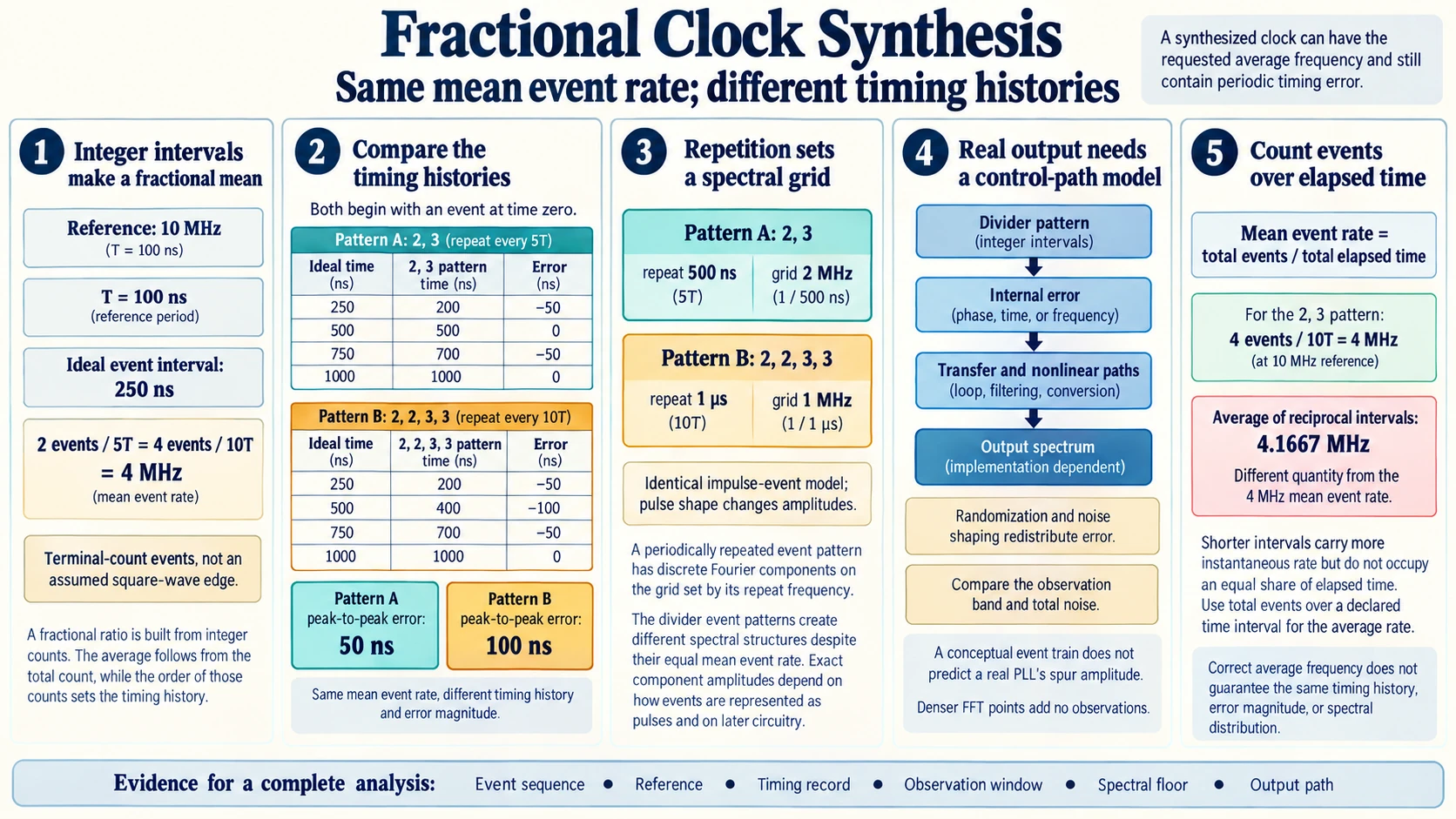
A synthesized clock can have the requested average frequency and still contain periodic timing error. Building a fractional ratio from integer counts sets the average through the total count, but the order of those counts sets the timing history. Repeating that history can create discrete spectral components.

Fractional clock synthesis therefore requires more than checking how many edges occur over a long interval. Two sequences can have the same mean division ratio while producing different error magnitudes, repetition rates, and spectral distributions.

The worked example emits an event after either two or three reference cycles. Its event stream provides an exact count and timing record. A particular phase-locked synthesizer needs an additional model connecting those internal events to its external output.

How fractional divider average follows from integer intervals

Let an exact reference have period T and frequency 1 divided by T. Define a divider event to occur after either two or three reference periods, according to a declared sequence. An output event is a terminal-count event here; no assumption is made that each event is one transition of a 50-percent-duty square wave.

For the repeating sequence 2, 3, there are two output events per five reference periods. Its mean event interval is 2.5T, giving average event frequency equal to 0.4 times the reference frequency. The mean division ratio is 2.5 even though no individual interval contains half a reference cycle.

If the reference is 10 megahertz, T is 100 nanoseconds. The event intervals alternate between 200 and 300 nanoseconds, while the desired ideal event interval is 250 nanoseconds. The long-term event frequency is 4 megahertz.

The frequency-counter guide supplies the rate interpretation needed for a fractional divider: a count divided by a declared gate gives the average event rate over that interval. It separates this rate from instantaneous endpoint behavior and reference error. That interpretation supports checking the total events across complete patterns here; the interval sequence still supplies additional phase-history information that the total does not preserve.

In the half-open interval from zero through, but excluding, 10T, the repeating 2, 3 pattern has events at zero, 2T, 5T, and 7T. Counting those four events confirms the average ratio. The endpoint convention fixes the count, while the interval record shows whether those events were uniformly spaced.

Trace cumulative departure from the ideal schedule

Start the first event at time zero. For the 2, 3 sequence, subsequent event times are 2T, 5T, 7T, and 10T. The ideal uniform schedule at the same average frequency is 2.5T, 5T, 7.5T, and 10T.

Subtracting ideal event times from actual event times gives errors of minus 0.5T, zero, minus 0.5T, and zero. The error repeats rather than accumulating without bound. At the 10 megahertz reference, the early-event displacement is 50 nanoseconds.

A constant shift of the schedule could center the error around zero, producing alternating departures of plus and minus 0.25T. That alignment change removes a fixed offset but does not remove the alternating variation. The peak-to-peak timing departure remains 0.5T.

Now use the repeating sequence 2, 2, 3, 3. It still contains two intervals of each size per ten reference periods, so its mean event interval and average event frequency are unchanged. Its event times are 2T, 4T, 7T, and 10T.

Against the same ideal schedule, its errors are minus 0.5T, minus T, minus 0.5T, and zero. The uncentered excursion is larger, and the pattern takes four output intervals to repeat rather than two. Correct average frequency has not guaranteed the same timing quality.

These cumulative calculations are more informative than looking only at the individual division values. Both sequences use exactly the same values and proportions. Their ordering changes the intermediate departure before the total timing error returns to zero.

How fractional spurs reflect repeated phase history

For the first sequence, the complete event pattern repeats every five reference periods. At a 10 megahertz reference, that is a 500 nanosecond repeat period, corresponding to 2 megahertz. The second pattern repeats every ten reference periods, or one microsecond, corresponding to 1 megahertz.

A periodically repeated waveform has discrete Fourier components on the grid established by its repeat frequency. The divider event patterns therefore create different spectral structures despite their equal mean event frequency. The exact component amplitudes also depend on how events are represented as pulses or passed into later circuitry.

The FFT-zero-padding guide explains an observation limit when assessing fractional spurs. A finite window spreads a component's spectrum, and a denser frequency grid can reveal that existing response without adding measurements. Its weak-tone comparison also requires the window, amplitude ratio, noise, and actual observation length. Those conditions help distinguish a physical periodic component from finite-record structure; that guide does not derive the divider's internal modulation or an oscillator's output spur level.

In a synthesizer, the fractional pattern can create periodic phase-detector error or another internal modulation that couples to the output. Its spectral manifestation then depends on the implementation and transfer paths. The conceptual event train does not establish a spur amplitude at an external oscillator output.

Correct average frequency constrains net event accumulation across complete patterns. It leaves the intermediate event departures visible in the cumulative record. Those departures can produce periodic spectral components when carried through an applicable output representation or implementation path.

An exact spectral example can be given for an ideal train of identical impulse events, rather than an unspecified clock waveform. Over the first pattern period of 5T, events lie at zero and 2T. Apart from the common normalization, Fourier coefficient k is one plus exp of minus j times two πk times two divided by five. The coefficient depends on where the events lie, not only on there being two of them.

The second pattern period is 10T, with events at zero, 2T, 4T, and 7T. Its coefficient is the sum of four corresponding complex phase factors on a different frequency grid. Both trains have the same average event rate, but their nonzero-frequency coefficients are not required to match. Finite pulse shape would multiply these coefficients by its own spectral envelope.

This explicitly defined ideal event spectrum supports the pattern argument without assigning an amplitude to an unspecified synthesizer output. Later circuitry can change those coefficients through its transfer and nonlinear behavior.

Texas Instruments gives a concrete fractional-division example in the LMX2594 documentation. The programmed N-divider value contains an integer part plus NUM divided by DEN, and a programmable sigma-delta modulator controls the fractional division. The document says resetting the modulator when R0 is programmed makes fractional spurs consistent. It also gives minimum-N restrictions dependent on modulator order and VCO frequency. These describe that device's control path; the terminal-count sequences of two and three in this article are independent mathematical examples, not valid LMX2594 programming settings or predictions of its output spectrum.

Randomization and noise shaping change the distribution

A deterministic short repeating sequence concentrates its error into a repeatable pattern. Rearranging intervals with a longer pattern can move the repetition structure. A randomized selection process can reduce simple coherent repetition while introducing broadly distributed fluctuation.

Such a process still needs a rule that produces the required long-term ratio. Merely choosing two and three unpredictably is not enough to guarantee every finite observation has exactly the desired average. Long-term mean, finite-window error, and cumulative timing bounds are distinct requirements.

Noise shaping uses structured state and feedback in the divider-control process to redistribute quantization error across frequency. Each declared integer interval remains an integer interval. The algorithm changes the frequency distribution and correlation of the resulting error.

A lower discrete line does not automatically mean lower total noise in every band. Error redistributed toward other frequencies can change integrated timing noise differently depending on the observation band and later filtering. A comparison should retain the band and metric rather than ranking one isolated peak as the complete outcome.

Randomized or noise-shaped algorithms can also retain periodic components under particular conditions. Their state rules, input ratio, finite precision, and implementation details matter. No general claim that a fractional architecture is spur-free follows from the method's name.

Keep implementation effects separate from the sequence

A real synthesizer can contain nonlinear conversion between internal error and output phase or amplitude. A periodic divider-control pattern may interact with those nonlinearities and produce lines not predicted by a purely linear transfer calculation. Conversely, filtering can suppress some pattern components before they reach the output.

The sequence analysis identifies candidate repetition and phase-history mechanisms. Establishing the actual spectrum requires the relevant transfer and nonlinear behavior, plus a measurement with enough resolution and a suitable reference. It does not provide a phase-locked-loop tuning procedure.

Different output representations also matter. A narrow pulse at each declared terminal count has a spectrum determined by pulse shape and event spacing. A separate oscillator controlled by those counts has its own dynamics. Treating them as identical would skip the very implementation path that determines the observed spurs.

A retained electrical waveform can show whether consecutive events follow the proposed interval pattern, provided the acquisition resolves their timing. SKU 18623303850 on the Unbranded ZT-703S Electrical Testing page is described with waveform export and storage. Those functions supply a possible acquisition context. The listing establishes no specified measurement noise floor, spectral sensitivity, or calibrated reference for an external synthesizer. The hypothetical 10MHz reference and 4MHz event rate in this article are not measured product results.

A time record should preserve enough consecutive events to show the candidate repetition and accumulated departure. A spectrum should identify carrier, offset frequencies, observation settings, and the measurement floor. Either record can fail to resolve a feature that the other reveals, so its limitations should stay attached to the claim.

A spectrum recorded through an audio path includes that path's timing and response. Four inputs with USB-C connectivity are described for SKU 1894010824 on the Focusrite AMZFCS4I4CR3X Red 4i4 Kit page. Its balanced outputs and recording accessories accompany this context for compatible audio. That description establishes neither direct measurement of the megahertz event trains here nor isolation of a separate synthesizer's internal divider error.

Frequency estimates for fractional clock synthesis should use total events divided by total elapsed time. Averaging the reciprocals of individual intervals gives a different result. For the 2, 3 sequence, the average of one divided by 2T and one divided by 3T is about 0.4167 divided by T, whereas the actual event rate is 0.4 divided by T. The shorter intervals carry more instantaneous rate but do not occupy an equal share of elapsed time. The total-count definition is the one used throughout this example.