Frequency counter accuracy: counts and reference bias

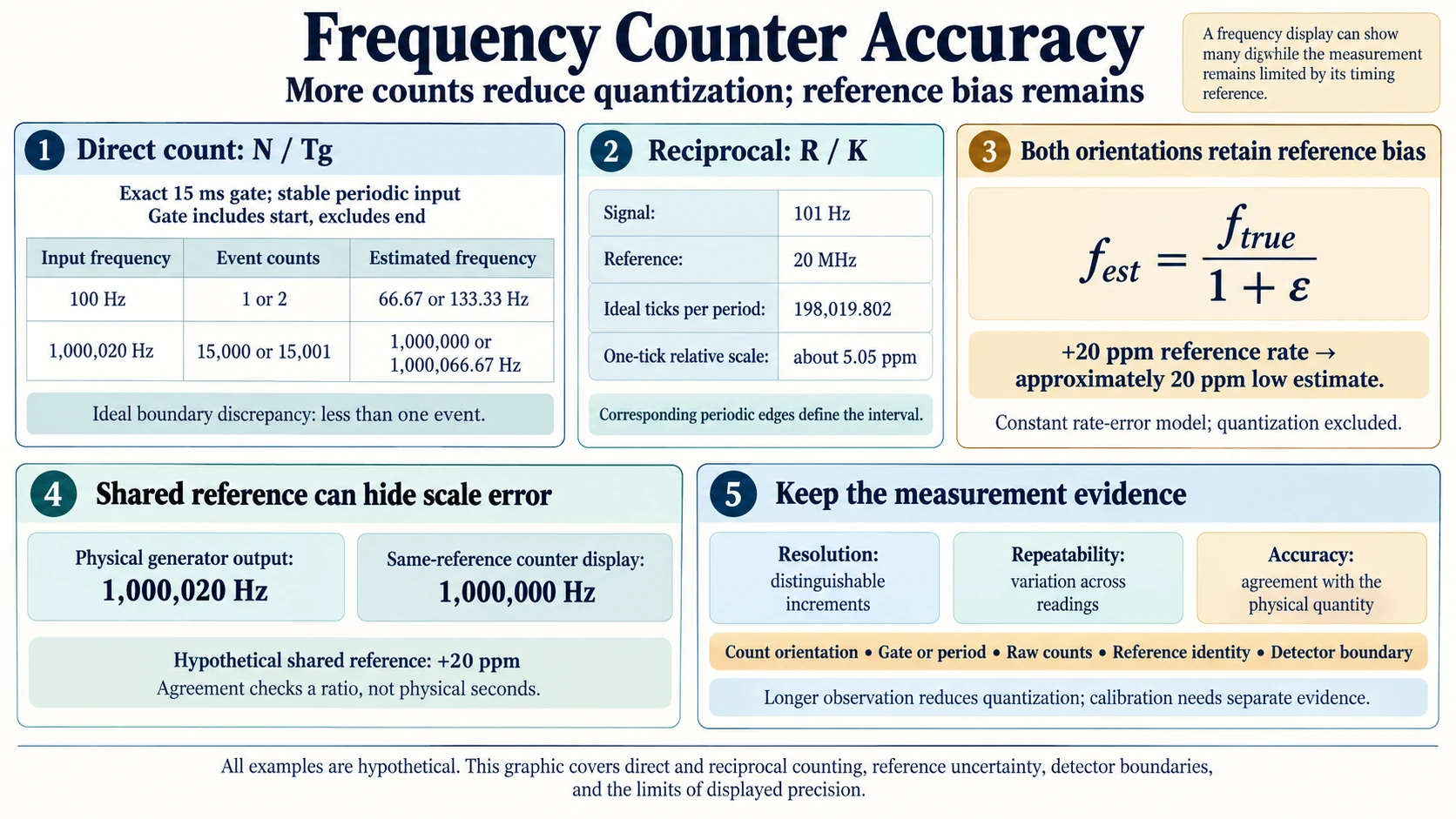
A frequency display can show many digits while the measurement remains limited by its timing reference. Counting more events or observing for longer can reduce one kind of uncertainty, but those operations do not establish that the reference seconds are accurate.

Frequency counter accuracy depends on the acquisition boundaries, quantization, and timebase as well as the signal being measured. Direct event counting and period-based measurement use the same reference in different orientations, which changes their useful resolution at different signal frequencies.

Direct counting measures input events during a reference interval. Period measurement counts reference ticks between input events. The calculations assume a stable periodic input and an appropriate detector; a changing signal needs an extended observation model.

How gate time sets the direct-count scale

In direct counting, observe N input events during a reference-defined gate of nominal duration Tg. The frequency estimate is N divided by Tg. The result is an average event rate over that gate, not necessarily the input's instantaneous rate at either endpoint.

For an ideal stable periodic input and an exact gate, use the half-open interval [start, end): count an event at the start and exclude one at the end. Moving that gate relative to the input events changes the integer total. For a noninteger ideal event total, the count is its floor or ceiling, and the discrepancy is less than one event.

The corresponding frequency-error magnitude from this ideal boundary quantization is less than one divided by Tg. A longer gate makes that bound smaller. It does not add fractional events to the counter or remove errors in the reference used to create the gate.

The monotonic-clock guide explains why gate time needs a rate contract as well as nondecreasing readings. Its hypothetical clock remains monotonic while reporting 300 physical seconds as 300.006 seconds under a constant positive 20ppm rate error. That example supports the distinction between clock progression and physical duration. The counting model still has to define which events enter the gate.

Real acquisition can have additional trigger, synchronization, or event-detection uncertainty. The less-than-one count statement belongs to the declared ideal boundary model, not every possible counter arrangement.

Linux documents a basic event-count primitive in its Generic Counter interface. Its example associates a pulsing input with an accumulating count: each rising edge triggers an increase. The selected edge condition determines which input transitions contribute. This describes counting behavior; the acquisition interval and its reference still have to be supplied before that total becomes a frequency estimate.

A concrete hardware example appears in Texas Instruments' TM4C123GH6PM documentation. In input edge-count mode, each selected input event increments or decrements the counter until the match value is reached. Down-count mode then stops and ignores further events until software re-enables it; up-count mode reloads zero and continues. That mode-specific behavior shows why the retained count and its acquisition limits need documentation. These timer primitives establish neither a named frequency counter's gate architecture nor its calibration.

The same count uncertainty has different relative impact

Take a hypothetical 100 hertz input and an exact gate lasting 15 milliseconds. The ideal event total is 1.5. Depending on alignment, the count is one or two, yielding estimates of approximately 66.67 or 133.33 hertz.

The two estimates straddle the true frequency even though the counting rule is correct. One divided by the gate duration is about 66.67 hertz, so the integer event scale is large relative to this low-frequency input.

For comparison, use a hypothetical input of 1,000,020 hertz with the same gate. Its ideal event total is 15,000.3. Counts of 15,000 or 15,001 give estimates of 1,000,000 or about 1,000,066.67 hertz.

The absolute count-derived frequency scale is unchanged, but its relative magnitude is much smaller at the higher input frequency. This explains why direct counting can provide useful relative resolution quickly for a high event rate and coarse results over the same short gate for a low rate.

When the ideal event total is an integer, the half-open gate gives that same count for every alignment in this ideal periodic model. The two examples above use noninteger totals to expose boundary quantization. Real detectors and gate circuits can add effects outside that model.

Observing longer can improve the count scale, at the cost of combining more signal history. If the signal changes during the gate, the result describes that larger observation interval. Increased numerical resolution and shorter response to changes are separate requirements.

How reciprocal counting reverses the measurement

For period-based measurement, let a nominal reference rate be R ticks per second. Count K reference ticks between two selected signal events. The estimated period is K divided by R, and the corresponding frequency estimate is R divided by K. This frequency formula requires positive K. A zero tick difference does not provide a finite reciprocal estimate under the stated count model.

The timer-input-capture guide supports the acquisition boundaries needed for reciprocal counting. Its constructed two-event comparison gives a 100-microsecond capture difference and a 95-microsecond handler-read difference because service delay changes. Those two events establish an interval; interpreting it as a period would additionally require a periodic signal and corresponding edges. The guide also explains how tick representation, acquisition delay, and retention affect the saved endpoints.

At a low input frequency, one signal period can contain many reference ticks. For a hypothetical 101 hertz signal and a 20 megahertz reference, the ideal one-period tick total is about 198,019.802. A tick-scale uncertainty is small relative to that count.

For large K, a change of one tick produces a relative frequency change approximately one divided by K. Here that scale is about 5.05 parts per million. The reciprocal formula is nonlinear, so an exact bound can be evaluated from the appropriate endpoint tick totals when needed.

For a very high signal frequency, one period contains fewer reference ticks and that orientation can become coarser. Measuring across several complete input periods can increase the reference count. The estimate then uses the known number of periods divided by the measured aggregate interval.

Both orientations compare event progression against a reference. Reversing the count does not create an independent physical second or remove event-boundary errors.

A biased reference affects both orientations

Let the actual reference rate be its declared rate R times one plus ε. Positive ε means its ticks occur faster than the nominal definition assumes. Ignore count quantization temporarily to isolate this bias.

A direct-count gate formed from a fixed number of reference ticks then lasts its nominal duration divided by one plus ε. The input contributes fewer events than it would over the nominal physical duration. Dividing that count by the nominal gate gives a frequency estimate equal to the true input frequency divided by one plus ε.

For reciprocal measurement, the faster reference puts more ticks inside one true signal period. Software divides the declared rate R by that larger count. The result again is the true input frequency divided by one plus ε.

The same reference bias therefore survives both orientations. For ε equal to plus 20 parts per million, the ideal estimate is approximately 20 parts per million low. The exact fractional bias is minus ε divided by one plus ε.

Increasing the direct gate or counting more periods can suppress relative quantization while leaving that systematic reference term. A more repeatable answer can consequently converge around a biased value.

The example assumes the reference error is constant during each measurement. If its rate varies, the relevant accumulated reference progression must be modeled over the acquisition interval. A single static correction factor may no longer describe the record.

Uncertainty terms also have different meanings. A deterministic reference-rate bound, a tick-quantization bound, and the observed spread of repeated readings should not automatically be combined as independent random variances. A combination rule needs a model for their distributions or a justified worst-case treatment.

A reference correction can reduce a known bias, but its own uncertainty remains part of the result. Repeat observations can characterize count variability under the tested conditions, while an independently supported reference relationship addresses the common scale error. Reporting which contribution each check constrains makes the final estimate reviewable.

Displayed precision is not a complete error budget

Resolution describes the measurement's distinguishable increments under its method. Repeatability describes variation across comparable repeated measurements. Accuracy requires evidence about agreement with the intended physical quantity and reference. A display can format more decimal places than the method supports.

Repeated identical counts can demonstrate stable behavior under those observations while leaving a common timebase bias unchanged. Conversely, varying counts may come from gate alignment even for a stable signal in the short direct-count example. Their interpretation needs the acquisition model.

The event detector can introduce another boundary. If input amplitude or edge slope changes the detection time, a period estimate can include that change. Counter arithmetic cannot distinguish it from event-time variation without additional signal and detector information.

An electrical trace can help examine which voltage crossing the detector admits. The Unbranded ZT-703S Electrical Testing listing, SKU 18623303850, includes waveform storage and export among its scope functions. Its nominal 20ppm timebase specification is a listing claim, not a calibration measurement. The listed multimeter frequency range ends at 999.9kHz, and the generator range reaches 1kHz. The hypothetical megahertz examples here describe no measured performance of this instrument or documented shared-reference arrangement.

A waveform record and a frequency number can support each other only when the relevant timebases and boundaries are understood. A signal produced by the same biased reference as the measurement can appear consistent without providing an independent reference check. For a declared generator whose nominal one-megahertz output scales with a shared reference that is 20 parts per million fast, the physical output is 1,000,020 hertz. A counter using that same reference reports the physical value divided by one plus the same rate error, giving exactly 1,000,000 hertz in the ideal model. The agreement verifies the shared ratio, not the physical second.

A recorded audio cycle has sample-index endpoints whose conversion to seconds requires the acquisition rate. USB-C connectivity and four inputs are described on the Focusrite AMZFCS4I4CR3X Red 4i4 Kit page, identified as SKU 1894010824. The listed recording accessories and balanced outputs accompany that audio-recording context. A period estimate from the record still needs its acquisition-rate evidence. The listing supplies no calibrated relationship to a separate frequency counter; agreement between them requires evidence about both timebases.

A retained measurement record can state count orientation, gate or period interval, raw counts, reference identity, and justified uncertainty terms. Those details allow a later analysis to distinguish a finer quantization scale from an independently verified reference. The formatted digits alone cannot reconstruct that evidence.