FFT zero padding: frequency-grid spacing and observation limits

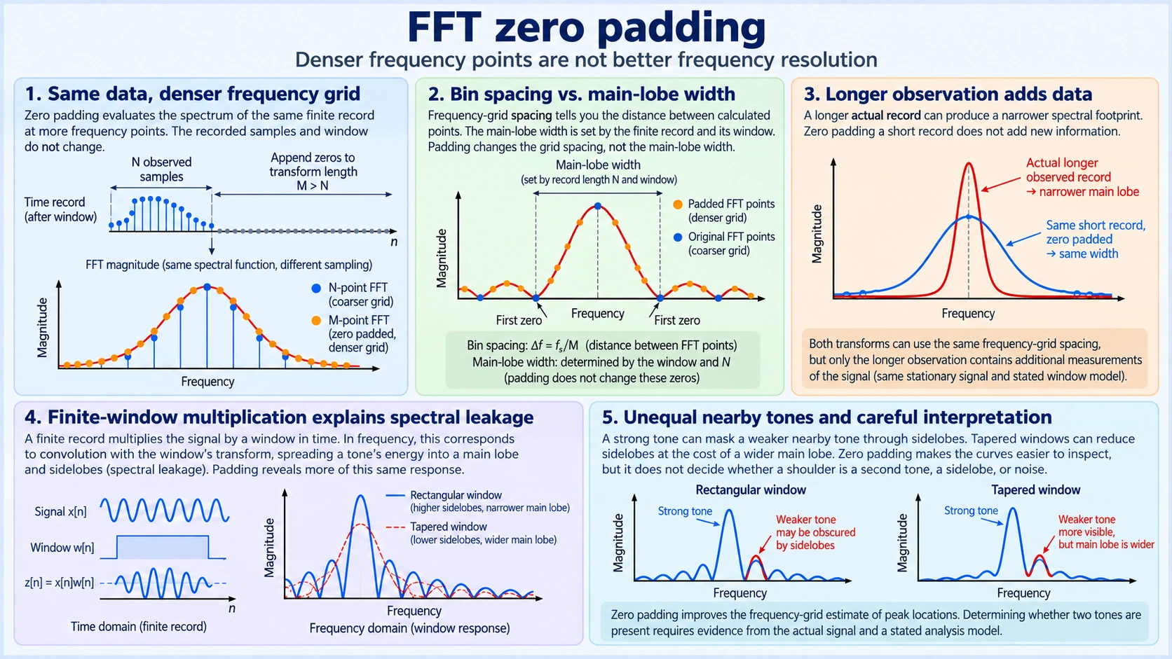
A short recording can produce an FFT plot with only a few points across a spectral peak. Append zeros to that recording, calculate a longer transform, and the peak acquires many more plotted points. Its maximum becomes easier to locate, and its outline looks smoother. The result is useful, but the extra points do not represent extra measurements.

FFT zero padding evaluates the spectrum of the same finite record on a denser frequency grid. The record still contains the same observed values and the same window. Two nearby tones that were difficult to distinguish do not become independently established merely because the software draws more points between the original bins.

To interpret the result, keep three quantities separate: the spacing of calculated frequency points, the spreading produced by the finite observation and its window, and the ability to identify signal components under the actual noise and amplitude conditions. They interact, but none is a complete substitute for the others.

FFT zero padding leaves the recorded data fixed

Suppose x[n] contains N uniformly spaced samples taken at rate f_s. Apply a window w[n] to obtain a finite sequence z[n] = x[n]w[n] for n from zero through N − 1. Define its continuous-frequency discrete-time transform as Z(ω) = Σ z[n]e^−jωn. Although the record contains a finite number of values, this expression can be evaluated at any frequency.

An N-point discrete Fourier transform evaluates that expression at ω = 2πk/N. An M-point transform of the same sequence followed by M − N zeros evaluates it at ω = 2πk/M. No additional nonzero terms enter the sum. Increasing M changes where the existing function is sampled, rather than changing that function.

For a hypothetical record containing 256 observed samples, a 256-point transform places points f_s/256 apart. Padding to 2,048 points places points f_s/2,048 apart. The eightfold increase in plotted density is exact. The record still contains only 256 observed samples, and its window still acts over those samples. Treating the longer transform as a longer recording confuses an array length with an observation.

That distinction should remain visible in stored analysis results. Record the observed sample count, sample rate, window, and transform length separately. A caption saying only “2,048-point FFT” cannot tell the reader whether the calculation used 2,048 measurements or 256 measurements followed by zeros. Both calculations are valid, but they support different interpretations.

Bin spacing and main-lobe width answer different questions

The frequency-grid spacing is Δf = f_s/M for an M-point transform. It tells you the distance between adjacent calculated values. It does not specify the width of a tone’s spectral footprint. That footprint is governed by the transform of the finite observation window and by the signal being analyzed.

For an unweighted N-sample rectangular record, the window transform contains a main lobe around its center frequency, with first zeros displaced by f_s/N on either side. Thus the first-zero-to-first-zero width is 2f_s/N in this particular model. Padding changes neither N nor those zeros. It supplies additional evaluations along the same lobe, making its shape easier to see.

Other windows have different main-lobe widths and sidelobe structures. A width defined at the first zeros differs from a width defined at a stated amplitude drop. Either can be useful if the convention is explicit. A claim about “resolution” without a window or a criterion leaves the reader unable to tell which width is being discussed.

Consider a single tone whose peak lies between the original FFT points. The largest unpadded bin can miss the true maximum of the finite-record spectral function. A padded transform samples closer to that maximum and reduces the frequency-grid error of a simple maximum-bin estimate. This improvement is real. It concerns locating a feature already present in the record’s spectrum; it does not narrow the window response or establish a second tone.

Longer observation duration adds data that padding does not

Compare two hypothetical measurements at the same sample rate. The first records 256 samples and pads them to 2,048. The second records 2,048 samples and uses an unpadded 2,048-point transform. Both plots have the same frequency-grid spacing. Their observed records differ by a factor of eight in length.

If the signal remains suitable for the comparison and the same window family is used, the longer observation can produce a narrower spectral footprint. It contains measured phase evolution over a longer interval. The shorter padded record contains no evidence about what happened after its last measured sample. Zeros in the array are arithmetic placeholders, not a statement that the physical signal became zero.

For two tones, the longer record can capture more of their relative phase change. Closely spaced frequencies produce a slowly changing relationship, so a brief segment may resemble one tone with a varying amplitude or phase. Extending the actual measurement can reveal behavior that the short segment did not constrain well. Evaluating the short segment at extra frequencies cannot supply that missing history.

Longer observation duration is not automatically preferable for every signal. A source may drift, switch, or cease to be stationary over the extended interval. In that case the longer record includes those changes, which must be interpreted rather than discarded as inconvenient. The benefit depends on whether the added measurements address the question being asked under a defensible signal model.

Finite-window multiplication explains spectral leakage

An FFT analysis begins with a finite portion of a signal. Multiplying a longer sequence by a finite window restricts its contribution to the observed interval. In frequency, that multiplication corresponds to convolution with the window’s transform. A tone that would have a sharp spectral line in an ideal infinite record therefore acquires the finite window’s shifted frequency response.

The main lobe is only part of that response. Energy also appears in sidelobes, whose levels and decay depend on the chosen window. This spreading is commonly called spectral leakage. It explains why an isolated tone can contribute values at many calculated frequencies, and why those values should not immediately be interpreted as many physical tones.

A rectangular record of a tone exactly aligned with an unpadded DFT bin provides a useful caution. At that grid, the tone’s window response has zeros at the other bin locations under the ideal stipulated conditions. The unpadded plot can therefore show one occupied bin. A padded plot samples between those zeros and reveals more of the response. Padding has not created leakage; it has made previously unsampled parts of the existing spectral function visible.

A tapered window changes that function. It can reduce some sidelobes while broadening the main lobe or changing other properties. The tradeoff matters because the analysis may need either a narrow central response or strong rejection of a large component’s contribution elsewhere. Appending zeros after windowing performs neither operation. It samples whichever response the selected window produced.

The interval used to acquire each sample is an earlier averaging operation. The sampling-aperture guide explains that interval's response and attenuation before a sample sequence exists. Distinguish it from observation duration, the span covered by the acquired record. The analysis window here selects and weights that record. Similar mathematics does not make acquisition response and finite-record analysis the same operation.

Unequal nearby tones expose the window tradeoff

Two equal tones can be easier to recognize than a weak tone next to a strong one. The strong tone’s window response may contribute more at the weak tone’s frequency than the weak tone itself contributes. A graph can then conceal the weak component even when the frequency points are closely spaced.

Suppose a strong tone and a substantially weaker tone are separated by a stated frequency difference. With a rectangular window, relatively narrow main lobes may coexist with sidelobes that obscure the weak tone. A suitable tapered window may lower those sidelobes enough to improve visibility, while its wider main lobe can make the closest separations harder to distinguish. Which effect controls the outcome depends on the separation, amplitude ratio, noise, and chosen window response.

FFT zero padding can make this comparison easier to inspect by supplying points across each window response. It cannot decide whether a shoulder is a second tone, a sidelobe, noise, or signal variation. That decision needs evidence appropriate to the component model, often including another observation or a fitted model whose assumptions and uncertainty are explicit.

Frequency estimation and component resolution should also be kept separate. A known single-tone model may permit a frequency estimate between FFT bins, particularly with good signal-to-noise conditions. A model that must decide whether one tone or two tones are present is a different inference problem. Neither problem is completely characterized by a universal reciprocal-duration formula or by the plotted grid spacing.

Use a controlled comparison before interpreting a smoother plot

Start with one saved sample array, one window, and one amplitude-scaling convention. Calculate the transform at two lengths, with the larger length obtained only by appending zeros. Compare the frequency-axis spacing and the locations of features on a common scale. The spectral outline should agree where the same frequencies are evaluated, allowing for numerical precision and the transform conventions used.

Keep normalization tied to the observed sequence and the desired reported quantity. Dividing blindly by the padded transform length can make a tone look weaker as more zeros are added. That is a scaling change, not a physical amplitude change. Window gain, one-sided versus two-sided presentation, and amplitude versus power conventions also need consistent treatment.

Next compare the padded short record with an actually longer record, if one is available. Preserve the original samples and record the additional acquisition interval. Any narrower response or newly apparent component now has an evidential basis in added measurements, subject to the window and signal assumptions. Label a simulation as a simulation if it supplies the extra data from a mathematical model.

Finally, inspect acquisition timing when interpreting spectral leakage. The sampling-clock-jitter guide shows how acquisition-time deviations alter recorded amplitudes through waveform slope. Those changes occur before the FFT. A denser frequency grid cannot undo the errors or supply the additional samples of a longer observation.

What equipment listings can establish

The ZT-703S combined instrument listing describes oscilloscope, multimeter, and waveform-generator functions, together with waveform storage or export. Those functions provide a possible context for recording and analyzing a waveform. The listing alone does not establish the exact saved sample interval, selected FFT window, padding behavior, or amplitude normalization needed for this comparison.

A recording made with the Focusrite Scarlett 4i4 fourth-generation interface bundle can supply the finite audio record for this analysis. Its catalogue entry lists USB-C connectivity, four inputs and four balanced outputs, together with recording accessories. Interpreting two close tones still requires the recorded samples and window, transform length and scaling; those details are not established by the hardware listing.

For a useful analysis record, retain the original measurements, acquisition rate, observed sample count, window, transform length, and plotting convention. Those facts explain what changed when the curve became smoother. Added frequency points improve inspection of the existing finite-record spectrum. Evidence for finer distinctions between physical components must come from the observed signal and a stated analysis model.