Equivalent-time sampling and the limits of composite traces

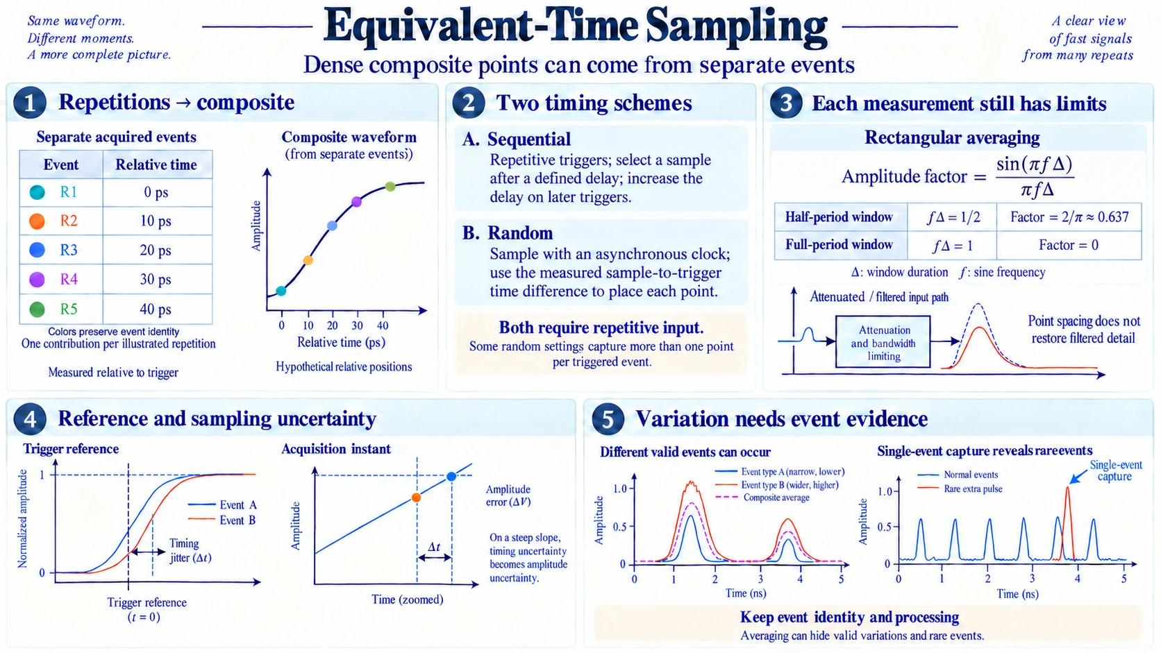
A waveform display can contain points spaced much more closely than the instrument acquired during any one repetition of the event. The instrument obtains the dense trace by collecting measurements at different relative times across repeated events, then arranging them on a shared time axis. This is the basis of equivalent-time sampling.

The assembled trace can be useful when the waveform repeats consistently and the timing reference is trustworthy. Adjacent displayed points may come from different physical events. A detailed composite trace is therefore not necessarily a recording of any one event from beginning to end.

A rare glitch, a changing pulse, or a nonrepeatable transient requires evidence tied to the event being studied. The display can describe a repeatable waveform model while failing to establish which variations occurred together in one repetition. Understanding the acquisition requires tracking both the relative time of each point and the event that supplied it.

Tektronix's XYZs of Oscilloscopes primer describes both random and sequential equivalent-time sampling and says both require repetitive input. Its sequential example takes a sample after a defined trigger delay, then increases that delay for subsequent triggers. Its random example samples with an asynchronous clock and places measurements according to their time difference from the trigger. The primer also notes that random sampling can collect more than one sample per triggered event under some settings. These descriptions support the two acquisition schemes here without assigning either scheme to a listed product.

Map displayed points back to their repetitions

Let repetition r have a trigger reference at time t_r. A sample collected at absolute time t_r + τ_r,m has a relative position τ_r,m within that event. The display can plot its measured amplitude at that relative position. If a later repetition supplies a point at a slightly different relative position, the instrument can place both points in the same composite trace.

In a hypothetical phase-stepped acquisition, the first repetition supplies a sample at relative time zero, the next at 10 picoseconds, and later repetitions at 20, 30, and 40 picoseconds. The resulting points are spaced 10 picoseconds apart on the display. They were not acquired 10 picoseconds apart in real elapsed time. Each may have been separated from the next measurement by a complete repetition interval.

The assumed picosecond values illustrate the mapping only; they are not specifications for a named instrument. A faithful data description would retain the event index, measured relative timing, and acquisition order. Without that information, a dense array of amplitudes can look like a single continuous record even though its points were collected over many events.

Repetition identity also explains what the trace cannot show. If the first repetition contains an early overshoot and the second contains a late undershoot, a composite can display both features. It does not follow that one repetition contained both. Joining neighboring points with a line can make the picture easier to read, but the line supplies no additional event history.

Different timing schemes can build the same kind of composite

One acquisition scheme deliberately changes the sampling delay after successive triggers. Each repetition contributes points at selected offsets, eventually filling a relative-time grid. A scheme of this kind depends on the event continuing to repeat while the offsets are collected. Its sequencing and trigger requirements must be assessed for the actual implementation.

Another scheme samples without forcing every measurement to the same relative phase. It measures the relationship between the sampling instant and the trigger, then assigns the sample to its relative-time position. Across repetitions, naturally varying relative positions can fill the display. The calculation depends on sufficiently accurate timing information; the displayed positions need not follow an ordered delay sweep.

Neither description establishes that all instruments implement either scheme in the same way. Some acquisition systems take more than one sample per repetition, average contributions within relative-time bins, reject acquisitions, or use other processing. The common feature is that points from multiple repetitions contribute to one relative-time representation.

For equivalent-time sampling, ask how each point's relative time is known, which repetition supplied its amplitude, and what processing combined the contributions. Those facts determine whether the composite supports a particular conclusion about the source. A point count alone leaves the acquisition history unspecified.

Analog bandwidth, real-time rate, and point spacing differ

The analog measurement path must respond to the signal before a sample value can represent it. A closely spaced composite grid cannot recover a fast waveform component that the analog input path has already attenuated or reshaped. The sampling scheme changes how observations are assembled; it does not automatically improve the response of the front end.

For repetitive waveforms, each acquired amplitude still depends on the temporal extent of its measurement. The sampling-aperture guide derives the response of a rectangular average: a window spanning half a sinusoidal period gives an amplitude factor of 2/π, while a full-period window cancels that sinusoidal component. Its subject is the measurement window, not assembly across repetitions. The comparison explains why collecting more relative-time positions cannot undo information lost within each acquisition window. The analog input path's amplitude, phase, and pulse response also remain necessary evidence; a scalar bandwidth endpoint leaves that complete response unspecified.

The real-time sampling rate describes the acquisition cadence within a continuous measurement record. Composite point spacing describes the distance between assembled relative-time positions. Dividing one by the other without explaining the acquisition can produce an impressive-looking number that obscures the actual experiment. A closely spaced composite may require many repetitions rather than one rapid series of measurements.

Likewise, a displayed edge with many points does not establish what happened between successive measurements of any one repetition. Under a stable repeated-waveform assumption, points collected on different repetitions can estimate that edge well. If the assumption fails, the same density can give a precise-looking representation of a changing source.

How trigger alignment establishes the shared time origin

Every composite point needs a position relative to an event reference. The reference can be a trigger derived from the signal, an external clock, or another identified timing event, depending on the acquisition. What matters is that the relationship between that reference and the feature of interest is known well enough for the intended comparison.

If the trigger reference moves relative to a repeatable edge, the edge moves on the relative-time axis even when its local shape is unchanged. Combining such acquisitions can broaden the displayed transition. In a bin-averaged display, the result can resemble smoothing. In a display retaining individual samples, it can appear as a band of scattered amplitudes. The rendering method affects the appearance, so it should be stated.

A trigger tied to the waveform itself can also remove or obscure some event timing variation. For example, aligning each repetition at a crossing may make that crossing look stable while another feature shifts relative to it. The display describes timing relative to the selected reference; it does not necessarily preserve the source’s timing relative to an independent clock.

The phrase trigger alignment should therefore refer to an explicit relationship, not a general assurance that the acquisition is synchronized. Identify the reference, the feature being compared, and the relative timing uncertainty. Otherwise, timing variation of the measurement system can be mistaken for waveform variation, or genuine event variation can be concealed by the alignment rule.

The sampling-clock-jitter guide supports the timing-uncertainty side of trigger alignment. It derives the small-error relation between local waveform slope, sampling-instant displacement, and amplitude error. It also separates the physical acquisition instant from a later delivery schedule. In a composite, the displayed relative-time coordinate and the instant that produced its amplitude both need evidence. Correcting the coordinate alone leaves an incorrectly acquired amplitude unchanged. The linked guide explains this acquisition-error mechanism; it does not specify an equivalent-time instrument's trigger algorithm.

Event variation in repetitive waveforms changes the composite

Suppose every repetition contains the same rising edge, but its amplitude alternates between two levels. Samples near the top of the pulse now come from two amplitude populations. Depending on display processing, the composite may show two bands, their average, or an inconsistent trace joining points from different levels. None of those displays establishes a pulse that followed the joined line during one event.

Another source might alternate between two pulse widths. An early sample sees the same high level in both cases, while a later sample falls inside the long pulse but outside the short one. The composite contains conflicting contributions at that relative position. This is useful evidence of variation if the acquisition preserves it. Averaging the values into one intermediate level can hide the underlying two-state behavior.

A rare extra pulse presents a further problem. If it appears on only one repetition, the acquisition may or may not sample its relative-time location during that occurrence. Missing it does not demonstrate that it never occurred. Capturing one affected point also does not necessarily establish the glitch’s complete duration, shape, or relation to other features of that same repetition.

The necessary repeatability depends on the question. A composite used to estimate a stable mean waveform can tolerate some variation if that variation and the averaging are acknowledged. A claim about the exact time history of one event requires event-specific evidence. The same acquisition can support the former while remaining insufficient for the latter.

Choose the acquisition for the event being studied

For stable repetitive waveforms, a composite can collect useful detail at relative positions that are sparsely sampled in any one acquisition. A suitable experiment keeps the waveform’s relevant properties and its relationship to the timing reference consistent throughout collection. It also accounts for the analog input response and the way points are combined.

For a nonrepeatable transient, the missing repetitions cannot be assumed into existence. Reconstructing its full history requires an acquisition that records that event with the needed temporal coverage and input response. A composite method designed around repetition does not become a single-event recorder because the final display is dense.

An intermittent problem may require both a stable composite to characterize the usual waveform and an event-specific capture to investigate departures from it. The composite supplies a reference shape; the capture establishes what happened during a particular occurrence. A comparison should retain that distinction in captions and conclusions.

A practical interpretation starts with the event model. Identify which features repeat and which changes matter to the question. Then identify the trigger reference and the acquisition's mapping from repetitions to displayed positions. If either is unknown, report that uncertainty alongside the waveform. Display density leaves those acquisition properties unspecified.

Separate the mathematical example from product capabilities

Waveform storage and export are among the functions described on the ZT-703S instrument page. The handheld combines a multimeter with an oscilloscope and signal generator. Retained waveforms provide a setting for asking which repetition supplied each recorded point. Its listed functions do not document the composite acquisition schemes explained here or establish the timing response used in the hypothetical example.

The Focusrite Scarlett 4i4 bundle listing describes a four-input USB-C interface, four balanced outputs, and recording accessories. Repeated audio events can illustrate why event identity matters when records are aligned and compared. That analogy does not establish an equivalent-time acquisition mode or high-frequency measurement capability in the listed interface.

To support an instrument-specific conclusion, consult the actual acquisition mode documentation and retained data. Preserve repetition identity where available, describe any averaging or point selection, and state the timing reference. A composite trace is most useful when its assumptions remain visible: detailed relative-time coverage can characterize a repeatable waveform, while evidence about one event must come from that event’s own measurements.