Clock frequency division: phase noise and edge displacement

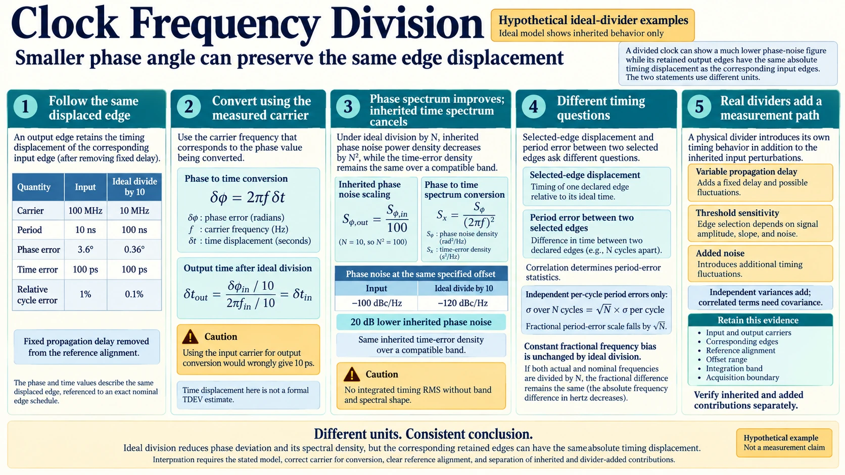
A divided clock can show a much lower phase-noise figure while its retained output edges have the same absolute timing displacement as the corresponding input edges. The two statements use different units. Phase measures an error relative to a carrier cycle; timing displacement measures it in seconds.

Clock frequency division reduces the carrier rate. In an ideal integer divider model, it also reduces inherited phase deviation by the division ratio. Converting that smaller phase deviation back to time cancels the same ratio, so ideal phase improvement does not automatically become proportional improvement in absolute edge timing.

Follow one declared perturbation through its phase and time descriptions. Real dividers also need an account of propagation delay and added fluctuations; the ideal inherited-error calculation covers neither automatically.

Describe one edge in phase and time units

Let a nominal carrier have frequency f and angular frequency ω equal to two πf. An edge displaced by a small time magnitude δt corresponds to a phase-error magnitude δφ equal to ωδt. A particular phase-sign convention may assign a late edge a negative phase; the magnitudes are sufficient for the scaling calculation here.

At 100 megahertz, the nominal period is 10 nanoseconds. A 100 picosecond timing displacement is one percent of that period. Its phase-error magnitude is two π times 0.01, approximately 0.06283 radian or 3.6 degrees.

The phase and time descriptions refer to the same displaced edge. They are not independent disturbances. Changing the carrier changes the number of radians assigned to a given number of seconds, even when the physical edge displacement remains unchanged.

Timing comparisons also need a reference. The hypothetical example uses an exact nominal edge schedule. A measurement against another imperfect clock would include that reference's timing behavior, so the observed displacement could not automatically be assigned entirely to the clock under test.

How phase noise scaling works under ideal integer division

Divide the input carrier by an integer N equal to 10. The nominal output frequency becomes 10 megahertz, and its nominal period becomes 100 nanoseconds. In an ideal phase-preserving division model for the inherited slow phase perturbation, output phase deviation is input phase deviation divided by N.

The 0.06283 radian input error therefore becomes about 0.006283 radian, or 0.36 degree, relative to the output carrier. The angular deviation is ten times smaller. It occupies one tenth as large a fraction of the now longer output cycle.

For the inherited phase-fluctuation spectrum under that model, phase power spectral density decreases by N squared. Expressed in decibels, the reduction is 20 times log base ten of N. Ideal division by 10 therefore gives a 20 decibel reduction in the inherited phase-noise figure under compatible measurement conventions.

The sampling-clock-jitter guide gives a phase-versus-time context for phase noise scaling. It explains that a constant acquisition-time offset corresponds to a phase displacement for a sine wave, and that the timing-to-signal effect depends on waveform frequency and slope. Those relationships support identifying the carrier and physical timing boundary before comparing units. The guide does not derive a divider transfer function or a phase-noise power density.

The phase-transfer statement needs its model boundaries. It describes inherited perturbations with a valid ideal division relationship. A real edge-selection system, high-offset behavior, and divider-generated noise may require additional treatment. The simple spectral scaling is not a universal description of all fluctuation frequencies and hardware effects.

NIST's Handbook of Frequency Stability Analysis defines time fluctuation x(t) as phase fluctuation divided by two pi times the carrier frequency. Its spectral definitions relate phase power density to time-error power density through the square of that same angular carrier frequency. The handbook also specifies its single-sideband phase-noise convention using half the phase-fluctuation density before the logarithm. These definitions support the unit conversions here; the ideal divider's inherited transfer relationship remains a separately declared model.

How time deviation follows after converting phase back to seconds

At the divided carrier, convert phase magnitude to timing displacement by dividing it by output angular frequency. The numerator is δφ divided by N, while the denominator is ω divided by N. Their ratio is δφ divided by ω, which is the original δt.

Numerically, 0.006283 radian divided by two π times 10 megahertz gives 100 picoseconds. The phase error decreased from 3.6 degrees to 0.36 degree, but the time displacement did not decrease from 100 to 10 picoseconds. It remains 100 picoseconds in this declared ideal example.

The timer-input-capture guide supplies an acquisition check for interpreting time deviation. Its constructed example preserves a correct event interval while the absolute capture values remain displaced by acquisition delay and quantization. It also separates the retained latch boundary from the later handler read. A divided-edge comparison likewise needs the actual measurement boundary and reference alignment. Here time deviation means absolute edge displacement in seconds, not a calculated formal time-deviation statistic.

A named time-deviation statistic can involve specific averaging and estimators. The single-edge δt calculation does not by itself provide such a curve. It establishes the unit conversion that prevents phase improvement from being mistaken for a proportional reduction of every time-domain quantity.

The longer output period also changes relative error. A 100 picosecond displacement is one percent of a 10 nanosecond input period but 0.1 percent of a 100 nanosecond output period. Relative cycle error improved, while the absolute number of seconds did not.

Retained edges and period errors ask different questions

An ideal divider can be viewed as retaining every Nth appropriate input edge, with a fixed propagation delay. After removing that fixed delay from the reference schedule, an output edge inherits the timing displacement of the selected input edge. It has not physically moved the selected event back onto its ideal time.

Output-period error compares two selected edges separated by N input cycles. Input-period error compares neighboring input edges. Those differences use different pairs of timing values, so their variances depend on the temporal correlation of the input fluctuation. The single-edge preservation statement does not say the two period-error distributions are identical.

For an explicitly hypothetical model with independent per-cycle period errors, the error over N cycles is their sum. Its standard deviation grows as the square root of N times the single-cycle standard deviation. Dividing by the N-times-longer nominal period reduces the fractional period-error scale by the square root of N.

That result requires the independence assumption. Correlated errors, periodic modulation, or a fixed rate bias give different relationships. It should not be applied automatically to a real oscillator merely because a divider counts cycles.

A constant fractional frequency bias also remains a constant fractional bias after ideal division. If both actual and nominal frequencies are divided by N, their fractional difference is unchanged. The absolute frequency difference in hertz decreases, but its parts-per-million value does not.

The spectrum conversion follows the same cancellation as the displaced edge. A phase power density Sφ converts to a time-error power density by dividing by the square of angular carrier frequency. Under ideal division, Sφ falls by N squared while that squared frequency also falls by N squared. The inherited time-error density therefore remains the same over the compatible band in this model.

For example, a hypothetical phase-noise level of minus 100 decibels relative to carrier per hertz at a specified offset would become minus 120 after ideal division by 10. That is not enough information to state an integrated timing RMS: the integration band and spectral shape are still required. Using compatible phase-noise conventions and the corresponding carrier converts both spectra into the same inherited time-error density.

Use the output carrier in the output phase-to-time conversion. If the input carrier is mistakenly retained after dividing the phase value by ten, the calculation reports an artificial tenfold reduction in seconds. That result comes from inconsistent conversion units.

Separate inherited and divider-added fluctuations

A physical divider can introduce variable propagation delay, threshold sensitivity, or other timing fluctuations. Those contributions require their own model or measurement. A fixed delay shifts the reference alignment; a fluctuating delay adds timing variation that the ideal inherited-phase result does not remove.

If inherited and added timing contributions are independent, their variances can be combined under that stated assumption. If they are correlated, a cross term is needed. Adding all RMS values directly or assuming independent power addition without evidence would obscure the actual relationship.

A phase-noise comparison should state both carrier frequencies, offset-frequency range, reference conditions, and any integration band. Dividing by a lower angular frequency when converting the output phase spectrum into time units is essential. Changing the integration band at the same time can create another apparent improvement unrelated to the simple division ratio.

Comparing a selected input edge with its divided output needs a retained record of both acquisition boundaries. Waveform export and storage are listed for the Unbranded ZT-703S Electrical Testing instrument, identified as SKU 18623303850. These electrical functions supply an observation context when the trace response supports the question. They establish no verified picosecond resolution or suitable noise floor for separating inherited and divider-added terms. The 100ps example is hypothetical, not a measurement made with this product.

A record of divided output alone also lacks the input comparison needed to assign noise to the divider. Measurements must identify which input edges correspond to output edges and account for reference and acquisition-path behavior. A lower carrier frequency alone supplies no measurement of timing noise.

A compatible audio recording carries its own acquisition conditions. The Focusrite AMZFCS4I4CR3X Red 4i4 Kit page identifies SKU 1894010824 and describes four inputs through a USB-C connection. Balanced outputs and recording accessories are also listed for that audio path. No independent picosecond measurement of the hypothetical 100MHz input or its 10MHz divided output follows from those features. An inference from the recording still needs its clock, conversion response and justified relationship to the external events.

Retain the paired input and output records, their carrier frequencies, corresponding edges, reference alignment, and applicable spectral band. The phase-to-time conversion can then be repeated with the output carrier and checked against the selected-edge timing. The record should identify which contribution was inherited and which divider-added behavior was actually characterized.