How arithmetic coding uses intervals and whole-message bit costs

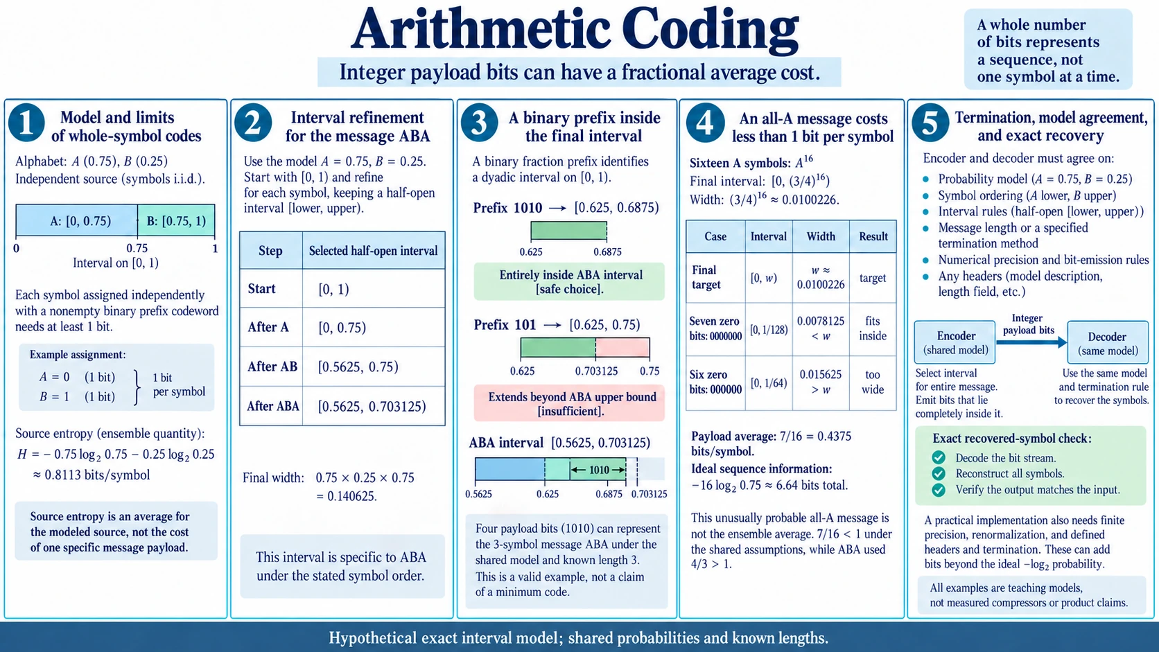
An encoded message contains an integer number of physical bits. Its average cost per source symbol can still be less than one bit when the encoder represents the sequence as a whole. Dividing that total bit count by the number of symbols gives a fractional average without assigning a fractional physical codeword to an individual symbol.

Arithmetic coding does this through repeated interval subdivision. A shared probability model determines how much of the current interval each next symbol receives. The observed sequence selects progressively smaller subintervals, and a final binary description identifies the selected interval.

The shared probability model, message-ending rule, and numerical conventions determine how the decoder interprets the emitted bits. The ideal fractional bit cost describes an efficiency target for that model. A complete implementation must also retain finite precision, headers, and termination under matching encoder and decoder rules.

Whole-bit symbol assignments limit a binary code

Consider a hypothetical source with symbols A and B, with probabilities 0.75 and 0.25. If each symbol is represented independently by a nonempty binary prefix-free codeword, both symbols need at least one bit. Assigning A = 0 and B = 1 costs exactly one bit per symbol, regardless of the probability imbalance.

The source entropy under this stipulated independent model is −0.75 log₂0.75 − 0.25 log₂0.25, approximately 0.8113 bits per symbol. The gap below one bit does not mean that A should receive a physical codeword of length 0.415 bits. It means that sequence-level descriptions can approach a lower average cost.

A block code can already overcome some whole-symbol rounding by assigning codewords to groups of source symbols. Interval coding offers another sequence-level mechanism. Its subdivisions correspond to probabilities without rounding every source symbol’s description to a separate whole number of bits.

The multiple-description guide offers a representation comparison for interval subdivision. In its fixed-field toy example, the same displayed string 101 means different bits in the two stream layouts. Stream identity and field conventions determine its interpretation. An interval decoder likewise needs the agreed model and symbol order to interpret its payload, but uses probability-defined regions instead of those fixed fields. The guide establishes no arithmetic-coding interval or termination rule.

David MacKay's Information Theory, Inference, and Learning Algorithms describes binary strings as half-open regions of the unit interval, then subdivides model intervals according to the next-symbol probabilities. The interval width becomes the modeled joint probability of the sequence. His encoder chooses a binary description whose entire region fits inside the message interval, and his decoder uses an identical predictive model. The worked source includes an end symbol; the examples below instead stipulate a known message length, so that stopping assumption remains explicit.

How interval subdivision refines a message

Start with the interval [0, 1), using an included lower endpoint and excluded upper endpoint. Allocate the lower 75 percent to A and the upper 25 percent to B. Thus A selects [0, 0.75), while B selects [0.75, 1). Both sides must use the same symbol order and endpoint convention.

For the message ABA, the first A selects [0, 0.75). Subdivide that interval with the same model. Its width is 0.75, so B selects the upper quarter, from 0.5625 to 0.75. The current interval is now [0.5625, 0.75).

The final A selects the lower three quarters of that interval. Its width before the selection is 0.1875; three quarters is 0.140625. Adding that to the lower bound yields the final interval [0.5625, 0.703125). Each step uses the previous interval, not the original unit interval.

The final width is 0.75 × 0.25 × 0.75 = 0.140625. Under the independent model, that product is also the assigned probability of the message ABA. Different messages of the same known length select nonoverlapping intervals under the stipulated subdivision rules.

This calculation is exact for the chosen rational probabilities. It describes an ideal interval model, not the internal integer arithmetic of a named file format. A practical implementation must define how it approximates and updates those boundaries.

A binary prefix identifies space within the final interval

A binary fraction prefix identifies a dyadic interval: a region whose width is a reciprocal power of two. The prefix 1010 corresponds to the interval [0.625, 0.6875). Every number with that initial fractional-bit pattern lies in that region, subject to a consistent endpoint representation.

That dyadic interval fits entirely inside the final ABA interval [0.5625, 0.703125). The four bits 1010 can therefore identify a region that decodes to ABA when the message length is known to be three and the model is shared. This is one valid illustrative description, not a claim of globally minimal formatting for the short message.

A shorter prefix can fail to identify a safe region. For example, 101 corresponds to [0.625, 0.75), which extends beyond the ABA interval’s upper boundary. Choosing an arbitrary numerical point inside the final interval and transmitting too few initial bits can therefore be insufficient. The emitted description must constrain the decoder enough under the actual termination rule.

To decode a representative value such as 0.625, the decoder first sees that it lies in A’s initial interval. It rescales within that interval, obtaining 0.625/0.75. This lies in B’s upper-quarter region. Rescaling within B’s selected interval gives a value in the next A region. After three symbols, the known length tells the decoder to stop.

The emitted prefix specifies an entire compatible region, not just the particular representative value used to explain decoding. Containment is what makes the example safe. A complete coding format may use a different bit-emission and termination procedure while implementing the same interval principle.

How fractional bit cost arises across a message

For sixteen A symbols under the same model, the ideal interval is [0, 0.75¹⁶). Its width is approximately 0.01002. The seven-bit prefix 0000000 identifies [0, 1/128), whose width is 0.0078125. That region fits inside the final interval.

With the length sixteen already agreed and the model shared, those seven illustrative payload bits identify the sixteen-symbol message. The payload average is 7/16, or 0.4375 bits per symbol. No individual physical bit was divided into a fractional object. The fraction arises from dividing the total integer payload length by the number of represented symbols.

The ideal negative-log probability of this particular message is −16 log₂0.75, approximately 6.64 bits. The seven-bit payload lies close to that quantity. It is below the source’s 0.8113-bit entropy per symbol because this particular all-A sequence is more probable than a typical mixture under the model. Source entropy is an ensemble expectation, not the exact cost of every message.

The short ABA example used four payload bits for three symbols and therefore did not beat a one-bit-per-symbol assignment. That is compatible with the mechanism. Integer endpoint selection and finite-message overhead matter, particularly for short messages. A useful efficiency claim states whether it concerns one payload, an expected cost over a source, or an asymptotic rate.

Termination and model agreement are substantive requirements

A final interval alone does not automatically tell the decoder how many source symbols to output. The encoding contract can provide a known length, a transmitted length field, an end-of-message symbol included in the model, or another defined termination mechanism. The chosen method consumes space or relies on shared context.

If an end symbol is added, the model’s alphabet and probabilities change. If a length field is transmitted, that field must itself be readable. Treating message length as free is acceptable only when it is already known through the stated surrounding format. The sixteen-A example makes that assumption explicit.

Encoder and decoder must also agree on symbol probabilities, symbol ordering, and how the model changes. An adaptive model can update after each decoded symbol, but both sides must start from the same state and apply the same update rule. Even a small disagreement can make later interval selections diverge.

The filter-bank guide provides an information-retention comparison for fractional bit cost. Its average and difference branches each hold one number per input pair; keeping both permits exact pair reconstruction, while the average alone loses a distinction. Reducing each branch's value rate therefore does not itself reduce the complete representation to half the information. The arithmetic example here instead counts integer payload bits across a whole source message. The filter-bank guide supplies neither a source probability model nor a bit-length claim for that message.

Finite precision changes how the ideal process is implemented

A literal interval becomes very small after many symbols, so a practical coder cannot retain arbitrary real-number precision indefinitely. Implementations use finite integer ranges, renormalization, and defined bit emission to continue the calculation. Their rounding and boundary rules must preserve a compatible interpretation for both encoder and decoder.

The implementation therefore needs enough range for its allowed symbol counts and probability representation. Extremely small symbol probabilities, frequency rescaling, and finite-width arithmetic are engineering choices rather than details that can be ignored after writing the ideal equations.

Headers, termination bits, and finite precision can raise the achieved cost above the ideal negative-log sequence probability. A mismatched model can raise it further because the encoder allocates too little representational space to events that actually occur. A correct decoder can still recover the message while compression efficiency is poor.

For a concrete assessment, compare the original symbol count with the entire encoded representation. Retain the model, its initialization, length convention, and numerical format. Decode the result and compare every recovered symbol with the input. A favorable ratio without an exact round-trip check does not establish lossless encoding.

Apply a model to saved electrical and audio records

An exported electrical record can supply symbols for a separately chosen software encoding example. The Unbranded ZT-703S Electrical Testing listing, SKU 18623303850, describes waveform-image storage and export in its handheld measurement context. The actual record still needs its native format and symbol interpretation identified. The listing provides no arithmetic-coding model or evidence that its own file uses this mechanism.

The Focusrite AMZFCS4I4CR3X Red 4i4 Kit, SKU 1894010824, connects by USB-C and provides four input channels. Its balanced outputs support monitoring and routing, and the bundle includes recording accessories. Before using a compatible signal recorded through the interface as coding input, identify the software values and their symbol alphabet, then select the probability model. The compression result belongs to the resulting software file and successful decoding; the listing names no interval coder or encoded size.

Save the emitted bits with the model, its initialization, the message-length convention, and the numerical rules used to encode them. The complete format can add header and termination costs to the illustrative payload. Decode every symbol under those same conventions and compare the recovered sequence with the input.