TCP retransmission timeout: delay estimates and recovery waits

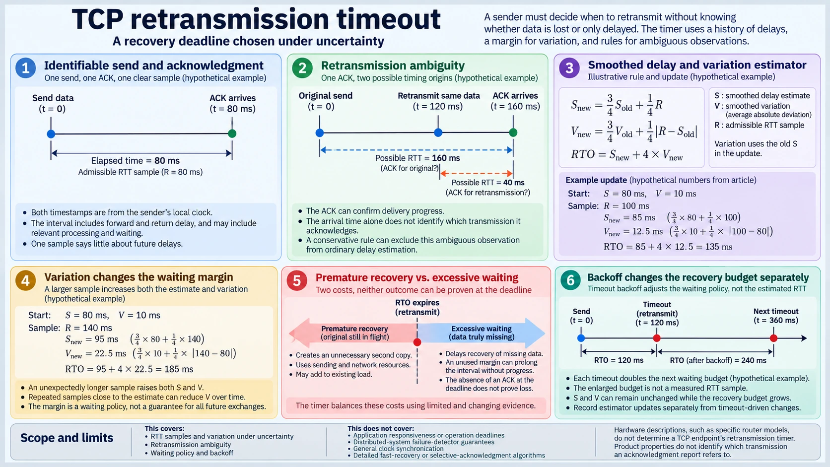
A sender waiting for an acknowledgment cannot immediately tell whether its data was lost or merely delayed. Retransmitting too soon can create an unnecessary second copy. Waiting too long can leave genuinely missing data unrecovered for an avoidable interval. The timer has to make a decision using a delay history that is incomplete and can change.

A TCP retransmission timeout is therefore a recovery deadline chosen under uncertainty. Choosing the deadline requires an estimate of ordinary round-trip delay and a treatment of its variation. It also needs a rule for observations whose transmission origin cannot be identified.

The examples here use explicitly stipulated timelines and estimator rules. They show how the information fits together without presenting their numerical settings as the defaults of every TCP implementation.

Start with an identifiable send and acknowledgment

Suppose a sender records a transmission at local time zero and receives an acknowledgment of that data at eighty milliseconds. The data was sent only once, and the report supplies the required progress information. Under those assumptions, the elapsed eighty milliseconds is an admissible sample for the round trip being measured.

The interval includes the outward journey and the return of the feedback. Depending on the measurement boundary, it also includes relevant processing and waiting between those events. It is not automatically a measurement of one link's propagation time.

Both timestamps in this example come from the sender's local clock. The sender does not have to infer the receiver's clock offset to measure its own elapsed interval. It does need a coherent definition of which transmission and acknowledgment delimit that interval.

One successful sample says little about the next exchange by itself. Queueing and other delays can vary, and the traffic conditions that produced the sample need not persist. A timer derived from that sample without a margin can expire during an otherwise successful exchange that simply takes longer.

An acknowledgment-arrival timestamp alone is insufficient to establish an admissible sample. The report must be related to a suitable transmission event under the measurement rule. Repeated delivery information should not automatically become a fresh independent sample of the same data's original journey.

How round-trip time estimation uses a changing history

Let S denote a smoothed delay estimate and V a smoothed measure of delay variation. For an illustrative estimator, choose a new sample R and update S as three quarters of its old value plus one quarter of R. Update V as three quarters of its old value plus one quarter of the absolute difference between R and the old S.

This definition uses the old delay estimate in the variation update. Using the newly updated estimate instead would implement a different rule. An explanation of a numerical trace should state this choice before calculating its results.

Begin with S equal to eighty milliseconds and V equal to ten. For an admissible sample of one hundred milliseconds, the new S is eighty-five. The absolute sample difference from the old S is twenty, so the new V is twelve and a half milliseconds.

Now stipulate a waiting budget equal to the updated S plus four times the updated V. That gives eighty-five plus fifty, or one hundred thirty-five milliseconds. The example combines a central delay estimate with a variation margin. It does not choose a fixed multiple of the latest observed delay alone.

V in this example is based on smoothed absolute differences. Calling it a variance or a standard deviation would describe a different statistic. Concrete implementations can also impose bounds and account for timer granularity; the stipulated arithmetic here does not select those implementation details.

A related measurement limit appears when round-trip time estimation is compared with network clock synchronization. That related topic explains why unknown forward/reverse delay differences can leave clock offset uncertain. The sender's elapsed interval here avoids that offset question by using one local clock, but it still does not reveal how the total delay divides between directions.

Variation changes the meaning of a waiting margin

A sender can encounter a longer sample even if its previous smoothed estimate was stable. Under the same illustrative rule, begin again with S equal to eighty and V equal to ten, but use a sample of one hundred forty milliseconds. The new S becomes ninety-five.

The sample differs from the old estimate by sixty. Updating the variation measure gives twenty-two and a half milliseconds. The stipulated budget then becomes ninety-five plus ninety, or one hundred eighty-five. The variation term reacts to the unexpected delay as well as the central estimate moving upward.

Repeated samples close to the estimate have a different effect. Their small absolute differences can reduce the smoothed variation measure over time. Under the budget rule, that reduces the variation contribution. The result depends on the history and update weights, not just the final sample written in a log.

The margin expresses a waiting policy. The fact that previous delays fit within it does not prove that every future delay will do so. A route or workload can change, and an estimator based on past observations cannot promise a bound on all later exchanges.

How retransmission ambiguity can spoil an apparent sample

Consider another timeline. The sender transmits data at time zero. With no qualifying acknowledgment yet observed, it sends the same data again at one hundred twenty milliseconds. An acknowledgment arrives at one hundred sixty.

That observation has at least two possible histories. The report might concern the original transmission after a round trip lasting one hundred sixty milliseconds. It might concern the retransmitted copy after a forty-millisecond trip. The arrival time alone is compatible with either history.

The acknowledgment can still establish delivery progress. The difficulty is identifying which send event should begin a delay sample. Measuring forty milliseconds assumes that the second copy caused the report; measuring one hundred sixty assumes that the first did. Without additional information, choosing either origin injects an assumption into the estimator.

This is retransmission ambiguity. A conservative sampling rule can exclude the ambiguous observation from ordinary delay estimation while still using its valid delivery information. Additional protocol information can sometimes disambiguate transmission timing, but that information must actually be available under the contract being analyzed.

Delivery feedback supplies useful positive evidence without settling every timing question. The acknowledgment-clocking guide follows how newly acknowledged data free sending allowance, which helps separate delivery progress from retransmission ambiguity. Its sending-account model does not identify which transmitted copy caused a particular report. Evidence that bytes arrived remains distinct from identifying a suitable delay-sample origin.

Compare premature recovery with excessive waiting

If a deadline expires while the original data is still progressing toward delivery, a retransmission can be premature. The second copy consumes sending and network resources without replacing a genuinely missing original in that history. On a busy path, additional traffic can also add to the existing load.

A sender cannot establish that this was the history merely from the absence of an acknowledgment at the deadline. The report might itself be delayed, or the original data might have been lost. The recovery decision is made before those possibilities are fully resolved.

A generous deadline can prolong recovery when data is genuinely missing. If data really is missing and no other applicable recovery mechanism acts, the sender waits longer before this timer initiates recovery. An unused margin can delay progress even though it avoided a premature second copy.

The estimator and waiting policy balance these costs using limited evidence. Increasing the margin reduces the chance that a delay like those represented by the history will trigger an early timeout, but it can extend recovery waiting. The right interpretation is a policy choice under stated assumptions, not proof that one deadline cleanly distinguishes loss from delay.

This timer concerns transport recovery. An application's own operation deadline asks a different question about when it stops waiting for its requested work. The transport timer should not be presented as a universal application-response deadline.

Backoff changes the recovery budget separately

Suppose the ordinary budget before a timeout is one hundred twenty milliseconds. Under a stipulated backoff rule, a timeout doubles the waiting budget for the next recovery attempt. The next budget is therefore two hundred forty, even if no new admissible ordinary delay sample has arrived.

If retransmission occurs at time one hundred twenty, a two-hundred-forty-millisecond wait places the next deadline at time three hundred sixty in this simple timeline. Another timeout could produce a four-hundred-eighty-millisecond budget under the same doubling rule. Implementations can have other limits and timer-management details; these values illustrate the separation of concerns.

The absence of feedback did not provide a measured round trip of two hundred forty milliseconds. Backoff changed how long the sender was prepared to wait during recovery. Treating the enlarged budget as an ordinary observed delay would confuse a control decision with a sample.

The smoothed estimate and variation state can remain unchanged while the recovery budget grows. Later, admissible observations can update ordinary estimation according to its separate rule. A log should record estimator updates separately from timeout-driven changes to the recovery wait.

Hardware descriptions do not select the endpoint timer

A router's advertised radio family does not define the TCP endpoint's estimator. The MSI RADIXAXE6600 tri-band Wi-Fi 6E router provides a networking-equipment example for a flow crossing a router. Its product description supplies neither the admissible sample history nor the timer weights and recovery deadline chosen by that endpoint.

The Nighthawk RS200 dual-band Wi-Fi 7 router is listed without an integrated cable modem. Those equipment properties describe a network component; they do not reveal whether an acknowledgment followed the original transmission or its later copy. That distinction requires the send/report timeline and whatever additional protocol evidence is available.

To interpret a TCP retransmission timeout, keep the sample history, its admissibility rules, and the current waiting policy visible. A sample with an identifiable origin can inform a smoothed estimate and variation margin. An ambiguous report can advance the delivery account without safely supplying that sample. Backoff can lengthen recovery waiting while leaving ordinary delay estimation unchanged.