Range-preserving digital smoothing: weights, state and edges

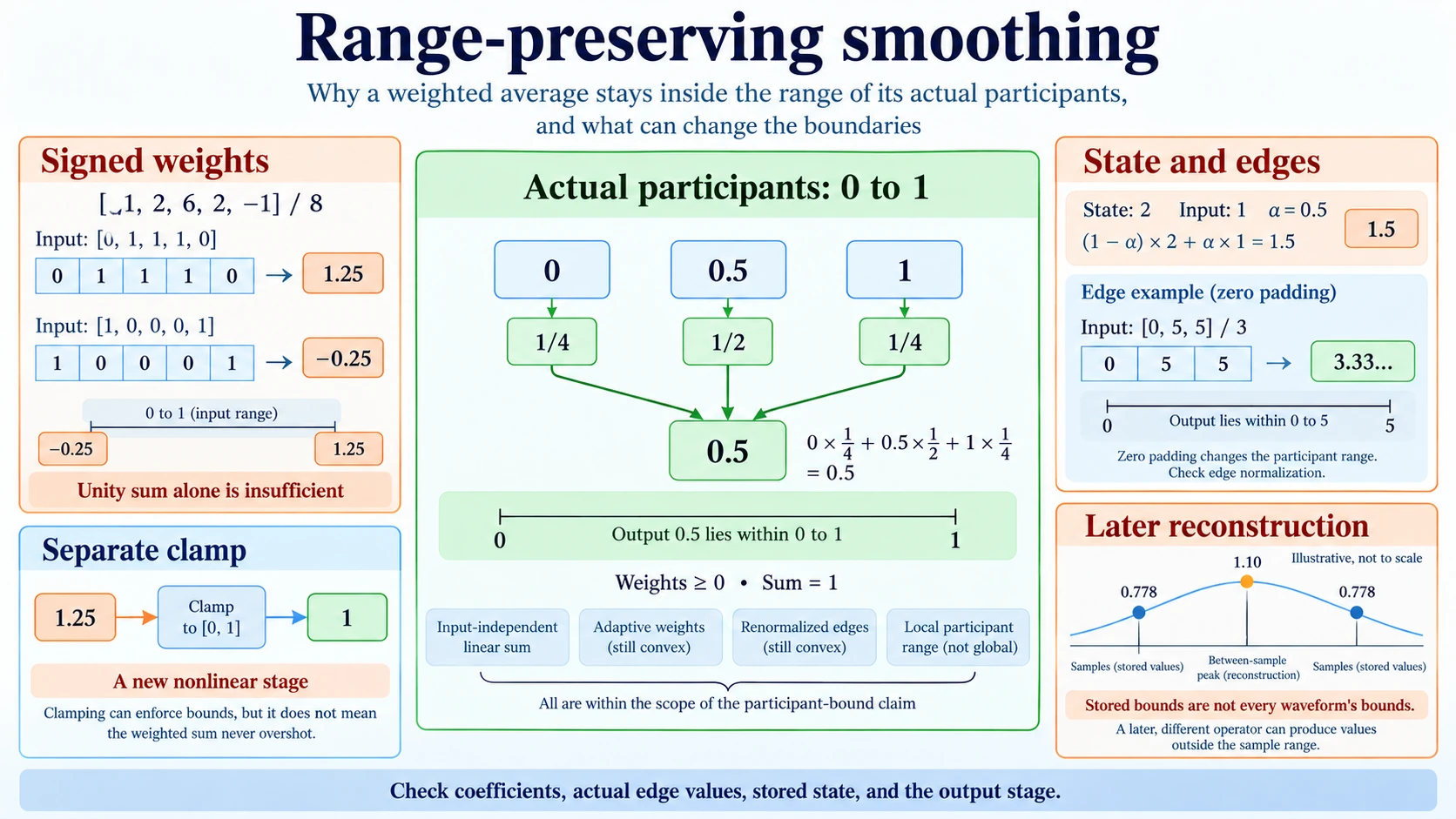
A filter can preserve a constant input while producing values above or below a changing input's range. range-preserving digital smoothing requires a stronger condition than coefficients summing to one. For a finite weighted sum, nonnegative normalized weights make the output a convex combination of the participating values.

Use exact arithmetic and stipulated kernels so that the guarantee can be checked directly. The examples do not address quantization, overflow, median selection, or safety of a measurement. They ask which values participate and which coefficient and state conditions support the bound.

Nonnegative filter coefficients give a finite-window bound

Let each participating input x_i lie between m and M. Let weights w_i be nonnegative and sum to one. The output is y=sum of w_i*x_i. Multiplying m less than or equal to x_i less than or equal to M by a nonnegative weight preserves the inequalities.

Sum those inequalities across the window. The lower side becomes m times the sum of the weights, and the upper side becomes M times that sum. Because the sum is one, m is less than or equal to y, and y is less than or equal to M.

The proof uses both assumptions. Nonnegativity keeps the inequality direction unchanged, and normalization makes the endpoint totals equal the original endpoints. The bound concerns the values that actually enter this output, including any boundary extension or prior state used by the implementation.

nonnegative filter coefficients with a unity sum therefore supply a direct finite-window guarantee. The weights can vary by position if each output's actual weights still satisfy the same two conditions. A nominal central kernel is not enough if edge processing changes them.

Nonnegative coefficients without normalization can also leave the input range. Three weights of one half have total weight 1.5. Applied to three values all equal to one, they produce 1.5. Unlike the signed-kernel example, this failure preserves coefficient signs and violates only the unity-sum requirement. Checking signs alone therefore supplies a different, incomplete test.

Digital smoothing overshoot with a unity-sum signed kernel

Stipulate the five weights [-1,2,6,2,-1] divided by eight. Their sum is one. Apply them to inputs [0,1,1,1,0], all within zero and one. The output is ten divided by eight, or 1.25, above the input maximum.

Apply the same kernel to [1,0,0,0,1]. The output is minus two divided by eight, or -0.25, below the minimum. The negative outer weights permit both examples despite the unchanged unity sum.

The kernel sums to one but violates the nonnegative-weight condition needed for the convex proof. A name such as smoother or a visually smooth response curve does not supply that missing inequality assumption.

digital smoothing overshoot can thus be a consequence of the operator, not evidence that a new input value existed. A reported output peak of 1.25 in the first example is generated from the stated zero-to-one window. Interpreting it as an observed source value would change the meaning of the data.

Constant preservation does not preserve every bounded sequence

For any constant c, a unity-sum weighted filter returns c times the coefficient sum, which is c. The negative-weight kernel passes that constant check. It nevertheless fails the two varying-input examples.

A test using only a constant sequence therefore proves less than a universal range claim. Test windows must expose the sign structure when assessing that claim. The mathematical proof, when applicable, provides the universal result without needing to enumerate every bounded sequence.

The zero-order-hold guide defines a full-interval output rule that selects the current sample until the next update. At an ordinary interior time in that model, one sample contributes with weight one and the others with weight zero. This gives a concrete comparison for nonnegative filter coefficients. The hold keeps that output within the stored sample range, while its separately discussed frequency response and later analog filtering do not follow from the range property alone.

A frequency-domain design objective can likewise address another property without asserting this value-domain bound. This article does not interpret general magnitude and phase response. It retains the actual weights so the range question can be answered on its own terms.

A recursive smoother also depends on its initial state

Consider y_n=alpha*x_n+(1-alpha)*y_previous. If alpha lies between zero and one, the two coefficients are nonnegative and sum to one. If both x_n and the previous output lie in [m,M], the same convex proof puts y_n in [m,M].

To extend that guarantee through the entire sequence, start with an initial stored output in [m,M] and keep every new input in the interval. Induction then supplies the result at each step. The initial-state premise cannot be omitted.

For example, let alpha=0.5, initial output two, and incoming input one. The first output is 1.5. It exceeds the input interval [0,1], although it lies within the range of its actual participants, which includes the initial value two.

Now set alpha=1.5 with initial output zero and new input one. The previous-output coefficient becomes -0.5, and the first output is 1.5. The convex condition has failed even though the two coefficients still sum to one. The formula's constant response does not restore the range guarantee.

The Lenovo IdeaPad FHD Touch listing specifies a 15.6-inch FHD Touch display, Intel Core i5-1334U, 16GB DDR4, and 512GB PCIe SSD. A trace table for the recursive example needs the initial value two beside the incoming value one and the computed output 1.5. Those numbers identify the enlarged participant range; the listed computer specifications supply no filter result.

Boundary padding changes the participating values

Suppose the original samples are all between five and ten, and a nonnegative three-point average uses zero padding at the edge. The padded zero lies outside the original interval. An edge output can fall below five while remaining inside the expanded participating range [0,10].

For a constant input five, averaging [0,5,5] equally gives ten divided by three. That result does not contradict the convex theorem. The theorem applies to [0,5], the range of that actual window, not to the unpadded sequence's single value five.

Replicating or reflecting existing values can keep padded participants within the original global range in this simplified setting. An extrapolated value can instead lie outside it. The boundary contract determines which set the proof bounds.

SciPy's convolution reference defines constant, reflected, replicated and wrapped extensions beyond array boundaries. Those definitions show how an edge can introduce a new participant or reuse an existing value. The arithmetic examples here use their declared extension rules; they do not report a particular software convolution as executed.

Edge renormalization needs its own coefficient check

Use positive kernel [0.25,0.5,0.25]. At the first sample, suppose only the center and right values are retained. Their original weights sum to 0.75. Keeping them unchanged sends constant five to 3.75, so the truncated operation does not preserve that constant.

Renormalize the retained weights by their sum. They become two-thirds and one-third, which are nonnegative and total one. The edge output is then a convex combination of the retained samples and stays within their range.

This rule requires a positive retained sum. It does not justify arbitrary handling of a negative-weight kernel or an empty set of samples. The actual edge weights, not the original interior weights, must support the claimed theorem.

The intersample-peaks guide constructs a sine wave whose stored magnitudes are about 0.778 while ideal reconstruction reaches 1.10 between samples. That comparison matters when interpreting digital smoothing overshoot: a bound on this specified discrete weighted sum does not automatically bound every later reconstructed waveform. The live guide explains that the ideal interpolation sum is not generally a weighted average with exclusively nonnegative weights. Its reconstruction model is therefore a different operator from the convex smoother proved here.

Clamping enforces limits through a different operation

An implementation can clamp a raw output to fixed limits m and M. That makes the final numeric result lie within those limits, but it does not show that the preceding weighted operator was range preserving. The raw overshoot remains a distinct intermediate result.

Clamping is nonlinear when it activates. With fixed limits zero and one, clamping 0.6 and clamping another 0.6 gives two values whose sum is 1.2. Clamping their sum gives one. The operations do not satisfy that additivity relationship.

It also discards information about excess magnitude. Raw values 1.25 and two both become one under the same upper limit. The final value cannot tell which raw excess occurred without a separate record. A weighted sum with fixed input-independent coefficients is linear in the full vector of participating values. The range proof itself also applies when the chosen weights depend on the data, provided each output uses nonnegative weights summing to one; that broader guarantee does not establish a linear overall mapping.

The ASUS Blue 14 FHD laptop provides a second computing-workspace example, identified in the catalogue as a laptop with a 14-inch FHD display. A raw-output and clamped-output table prepared in that workspace should retain 1.25 and one in separate fields. Their difference shows which stage enforced the bound. Those calculations are stipulated examples; no filtering result on the linked computer was measured.

Verify the range claim for the operator actually used

Specify whether the claimed interval is global or local. If a complete sequence lies between zero and ten but one window contains only values between five and six, a convex output for that window stays between five and six. Clamping another operator only to zero and ten supplies a weaker bound. A raw value seven survives that global clamp while remaining outside the local window range.

The interval can be chosen for each output from its participating samples when the proof conditions hold there. For a recursion, those participants include the previous state, so an input-only local interval may be too narrow. A bound that changes meaning between interior windows, padded edges, and recursive startup can produce confusing results even when each arithmetic step is correct. Name the participant set beside the guarantee.

Record the actual coefficients, their signs and sum, participating samples, initial state, and boundary rule. For a recursive claim, retain the state induction premises. For an edge claim, inspect the edge weights or extension values directly.

If the convex conditions hold, the inequality proof gives the stated bound. If they do not, a unity sum or passing constant test does not fill the gap. A clamped result supplies a limit from the clamp, with its separately defined nonlinear consequences.

The negative-weight examples reach 1.25 and -0.25 from zero-to-one inputs. The recursive and padded examples exceed a narrower input-only interval because their actual participants differ. The first checks are the coefficient signs and sum, followed by the actual edge values and stored state admitted into each output.