Digital filter approximation objectives: worst-case and squared error

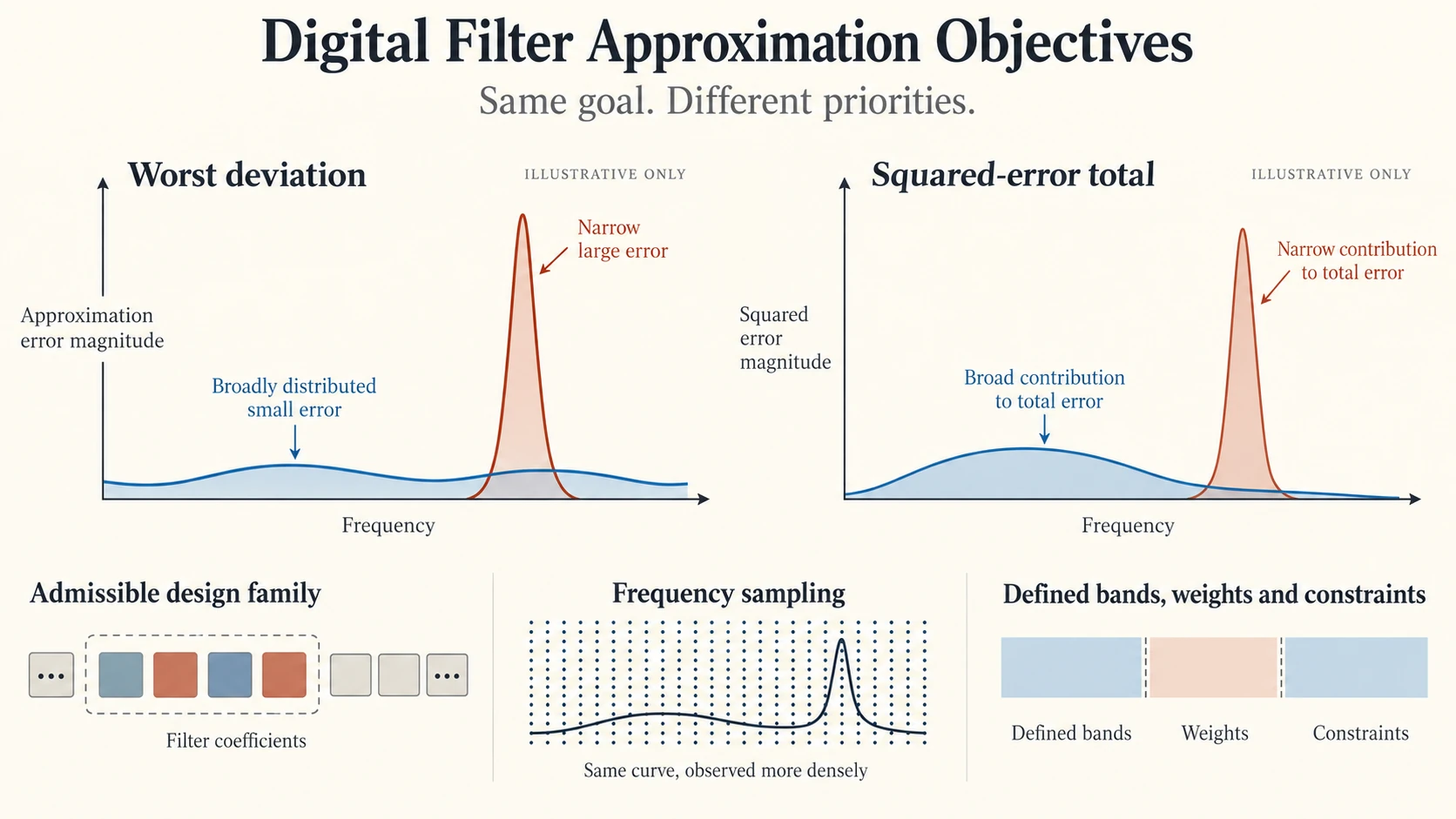
With a fixed target response and coefficient budget, digital filter approximation objectives determine how the design charges error. One criterion limits the largest deviation; another minimizes accumulated squared deviation. They can prefer different error shapes even when the target and allowed design family are unchanged.

Use a stipulated low-pass target with gain one in a pass region and zero in a stop region. Leave a specified transition region outside the scored approximation regions. The discussion uses idealized error profiles to inspect objective meaning; it does not report a verified filter or an optimal result from a software package.

Define the target, admissible coefficients, and scored regions

Let the admissible designs have a fixed number N of real coefficients, together with any additional family constraints the design contract explicitly requires. The frequency response follows from those coefficients. A coefficient vector outside that set is not a candidate merely because its error curve looks attractive.

Define error as the realized response quantity minus the desired response quantity on the scored regions. The quantity might be a specified real response component or another expressly chosen representation. Comparing objectives requires the same error definition for both.

The pass and stop regions determine where error is charged. The excluded transition region can have behavior that the objective does not penalize. If the application needs a bound there, that requirement must be added rather than inferred from good scores elsewhere.

Also identify the frequency coordinate and measure used by an integral. A continuous integral, a sum on a sampled grid, and an average normalized by band width need not have the same numerical interpretation. A design claim should name which was actually optimized and checked.

Compare a broad small error with a narrow large error

For objective arithmetic, normalize the total scored frequency measure to one and use unit weights. Profile A has absolute error 0.1 across that measure. Profile B has absolute error 0.5 over a subregion of width 0.01 and zero elsewhere.

A's maximum absolute error is 0.1, while B's is 0.5. A wins the worst-case comparison. A's integrated squared error is 0.1 squared times one, or 0.01. B's is 0.5 squared times 0.01, or 0.0025. B wins the integrated comparison.

The two comparisons are arithmetically consistent. A spreads smaller error broadly; B concentrates larger error into a narrow region. The integral makes the width of that region matter, while the maximum only asks about its highest charged deviation.

These rectangular profiles are deliberately simplified illustrations of objective costs. They are not claimed frequency responses of two particular N-coefficient filters. To choose between actual filters, compute each realized error from an admissible coefficient vector and evaluate the defined objectives on it.

Worst-case weighting and equiripple filter design

With nonnegative weights, a weighted minimax objective can be written as the largest value of w(f) times absolute error across the scored regions. If a band receives a larger weight, a smaller error there can produce the same charged maximum as a larger error in a lower-weight band.

For suitable approximation problems, equiripple filter design balances extremal weighted errors under the minimax criterion. That phrase concerns the charged approximation pattern within its stated design problem. It does not guarantee equal unweighted deviations everywhere or a particular response in excluded regions.

Weights therefore express priorities among the included frequencies. If the stop region's weight is four and the pass region's is one, a stop error of 0.025 and a pass error of 0.1 have equal weighted magnitude. This is an objective relationship, not an independently required bound on every candidate.

The FFT zero-padding guide provides a sampling comparison relevant to equiripple filter design. It explains how a longer transform evaluates the same finite-record spectrum at more frequency points without changing the underlying function. A denser evaluation grid can likewise reveal more of a candidate filter's error curve. The grid alone supplies neither a new coefficient vector nor a proof of the continuous maximum. The linked guide discusses finite-record spectra; it does not derive minimax filter designs.

Least-squares frequency response charges the area of squared error

With nonnegative weights, a weighted least-squares objective can instead integrate w(f) times the square of the error. The amount of frequency space carrying a deviation contributes to the total. A narrow peak can be cheaper than a broad lower error, as the stipulated profiles show.

The numerical weights need their own convention. With the objective just defined, weight four multiplies the squared error by four. That is equivalent to multiplying error amplitude by two before squaring, not by four. In the minimax formula above, weight four multiplies absolute error by four.

least-squares frequency response design therefore should not inherit a minimax weight table without checking its meaning. If the intent is the same amplitude scaling before squaring, the least-squares coefficient multiplying error squared would use the square of that amplitude weight.

The same weight change can reverse the illustrative integral ranking. Give B's narrow 0.01-wide region weight ten and the remaining 0.99 measure weight one. B's weighted squared total becomes 0.025. A's becomes 0.1 squared times (ten times 0.01 plus 0.99), or 0.0109. A now wins this weighted integral comparison. The profiles did not change; the charged priorities did.

That calculation should not be read as a recommendation to select weight ten. It demonstrates why weights belong to the problem statement. A design report that omits them can hide the premise responsible for its preferred candidate. An application must justify the frequencies it treats as more costly and the weighting convention through which it expresses that cost.

Band width matters as well. Two regions with the same weight but different widths can contribute different total error even when their local squared deviations are similar. An objective that averages each band's error before combining them would encode another priority contract.

A value-range requirement can add a coefficient constraint to a least-squares frequency response problem. The linked smoothing guide proves that nonnegative weights summing to one keep a finite weighted output within its participating input range. Its signed unity-sum example reaches 1.25 from inputs between zero and one. A frequency-response fit by itself supplies no such sign condition. If range preservation is mandatory, impose the relevant coefficient restrictions when defining the admissible family and then compare objective values within that family.

Hard response constraints differ from penalized error

Add a mandatory condition: absolute error must never exceed 0.2 on the scored regions. Profile B fails that condition despite its smaller integrated squared score. Profile A passes it in the simplified example.

If the bound is hard, reject B before ranking feasible candidates by their least-squares objective. Making a region expensive in the objective can encourage a smaller deviation there, but a finite penalty does not automatically enforce an exact upper bound.

The converse distinction also matters. A candidate satisfying the hard bound can still have poor integrated error compared with another feasible candidate. Feasibility and preference are separate decisions. The design contract should state both when the application needs both.

The Lenovo IdeaPad FHD Touch laptop is listed with a 15.6-inch FHD Touch display, 16GB DDR4 and a 512GB PCIe SSD. A comparison table in that computing workspace can keep maximum error, squared-error integral and hard-bound feasibility in separate columns. For the stipulated profiles, B's better integral still leaves it infeasible when the 0.2 bound is mandatory. This is objective arithmetic, not a measured filter design on the laptop.

An optimality statement belongs to the complete problem definition

A claim of optimum identifies the admissible coefficient set, target, scored regions, weights, objective, and any hard constraints. Changing a band edge or weighting convention changes the problem. A previous optimum does not automatically remain optimum for the new definition.

Likewise, an algorithm's returned coefficient vector needs evidence about the objective and constraints it actually achieved. A method described as minimax does not turn an unobserved result into a verified maximum-error bound. This article's profile calculation supplies no coefficient vector and makes no optimal-filter claim.

SciPy's documentation for signal.remez describes minimizing the maximum error in the specified bands, while signal.firls describes minimizing integrated weighted squared error in its stated design family. These definitions support the comparison here. The numerical examples are stipulated error profiles; no package invocation or optimal coefficient vector was calculated for this article.

A sampled check can miss a peak between its samples. A continuous-region bound requires an appropriate check for that claim. If only a grid was evaluated, record the grid and report the narrower observation rather than silently turning it into a continuous optimum.

Application requirements can remain outside either objective

Response error is not the only possible application requirement. Delay, behavior in the excluded transition region, or another response quantity may need separate treatment. A smaller approximation objective does not prove that those requirements were satisfied.

An equal numerical deviation can also have different application meaning in the two bands. A pass-region deviation changes the desired transmitted component, while a stop-region deviation leaves a component the target intended to suppress. The unweighted objective treats equal error magnitudes alike because that is its definition. Distinguishing their consequences requires an explicit priority or constraint rather than an assumption that the score already contains it.

Choose the criterion by the failure the application needs to control. If a narrow high deviation is unacceptable anywhere in a region, a maximum-error criterion or a hard bound directly reflects that concern. If accumulated squared deviation is the intended cost, the integral provides another meaningful comparison.

The ASUS Blue 14 FHD product page describes a laptop with a 14-inch FHD display, which can be used to view plots of the two profiles. The listing supplies no approximation accuracy or computation benchmark. Keep the idealized curves labelled as objective illustrations rather than presenting them as measured designs run on the listed computer.

For profiles A and B, the maxima are 0.1 and 0.5 while the integrals are 0.01 and 0.0025. The reversal follows from the objective definition. A useful filter comparison retains that definition, its weights and regions, and the application constraints before declaring one distribution of error preferable.