Cabinet hardware sample cost: when an order check pays

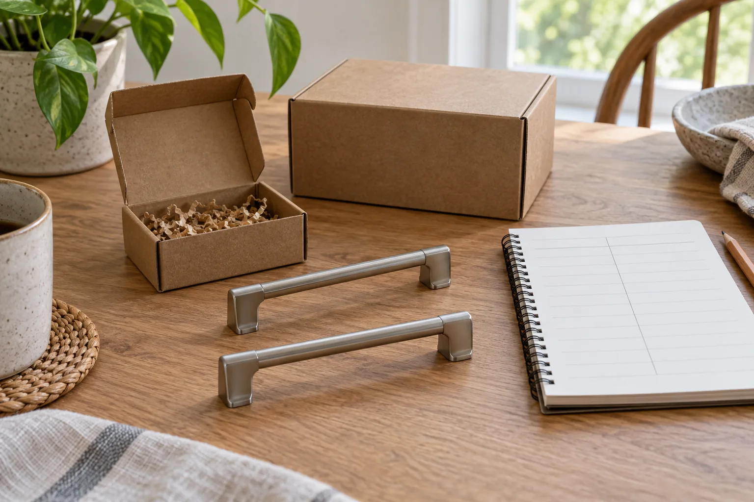
Cabinet hardware sample cost is an extra expense that can be worthwhile when it avoids committing money to an unsuitable full order. Whether it reduces expected spending depends on the sample overhead, the money exposed in the large order and an assumed chance of an unsuitable result. A paper calculation can show where that trade changes direction. It cannot supply the missing chance or establish that a real sample predicts a complete order.

The Amerock Hybridize cabinet pull offer describes a 25-pack. Its actual name and description identify Oil-Rubbed Bronze, although the URL contains different finish wording. The Emtek 86710 Warwick cabinet pull offer identifies a separate model. Neither offer establishes the sample sale, trial arrangement or hypothetical prices used below. Confirm any real sampling option with its supplier before budgeting for it.

Define the sample order budget before comparing strategies

For this sample order budget, imagine an already specified furniture-hardware project. Every amount is invented and expressed in the same currency units. The required full lot costs 120 units. A different, suitable alternative would cost 150. Obtaining and assessing a separate evaluation sample adds 12 units, including every sample expense assumed in this model. The 12 is an overhead paid in addition to a later full order.

Assume the sample cannot count toward the final quantity, earn a credit or be sold afterward. Also assume it perfectly reveals whether the first design will be suitable for the entire intended project. These stated assumptions keep the arithmetic simple. They describe the fictional decision only. An actual small item may leave finish variation, quantity, mounting or other requirements unanswered; no assessment method is supplied here.

There are two possible outcomes in the model: the first design is suitable, or it is unsuitable. Both strategies finish with the same required quantity of suitable hardware. In the unsuitable outcome, both obtain the 150-unit alternative. Initially, assume money spent on an unsuitable full lot cannot be recovered. These conditions keep the comparison about expenditure for the same completed requirement.

Write the spending in each outcome

Ordering the full first lot immediately costs 120 units if it proves suitable. If it proves unsuitable, the buyer has spent 120 and must spend another 150 on the alternative. That outcome totals 270. The unusable lot remains in the fictional buyer's possession with no recovery value in this first calculation. The alternative's cost is added only in the unsuitable outcome.

Starting with the sample costs 12 units regardless of its result. A suitable result is followed by the 120-unit lot, producing a total of 132. An unsuitable result is followed directly by the 150-unit alternative, producing 162. Sample-first spending therefore lies between 132 and 162 in this two-outcome model. Immediate full-order spending lies between 120 and 270.

Compare matching outcomes before averaging. When the first design is suitable, sampling costs 12 more: 132 instead of 120. When it is unsuitable, sampling costs 108 less: 162 instead of 270. The second difference is the avoided 120-unit lot minus the 12-unit sample overhead. Calling the sample an automatic saving would discard the suitable outcome, where its overhead buys no expenditure reduction.

Expected purchase expenditure needs an assumed probability

For expected purchase expenditure, give the unsuitable outcome an invented probability of twenty percent. The suitable outcome then has eighty percent. These are arithmetic inputs, with no survey, failure record or observation behind them. The expected amount is the sum of each outcome's spending multiplied by its assumed probability. The calculation preserves the two outcomes even though its answer is a single number.

For the immediate full order, multiply 120 by 0.80 and 270 by 0.20. The contributions are 96 and 54, adding to 150 units. For sample first, multiply 132 by 0.80 and 162 by 0.20. Those contributions are 105.60 and 32.40, adding to 138. Under precisely these assumptions, the sample strategy has twelve units less expected expenditure.

Neither strategy actually spends its expected amount in this example. The immediate buyer spends either 120 or 270; the sampling buyer spends either 132 or 162. The figures 150 and 138 are weighted averages of possible outcomes. They cannot serve as a promised invoice or a guarantee that one household will save twelve units on one project.

An imagined collection of one hundred such projects gives another view of the same arithmetic. Assign eighty to the suitable outcome and twenty to the unsuitable one. Immediate full ordering totals 15,000 units across that supplied collection; sampling totals 13,800. Dividing each total by one hundred recovers 150 and 138. This constructed collection illustrates the weighting and predicts no actual set of purchases.

Find the point where sample overhead balances avoided loss

Now lower the invented unsuitable probability to five percent. The immediate strategy's expected expenditure is 0.95 times 120 plus 0.05 times 270, giving 127.50 units. Sampling gives 0.95 times 132 plus 0.05 times 162, or 133.50. The same twelve-unit sample now increases expected expenditure by six units. Changing the assumed probability changed the comparison without changing any outcome's bill.

At a ten-percent unsuitable probability, both strategies have expected expenditure of 135 units. For immediate ordering, that is 108 plus 27. For sampling, it is 118.80 plus 16.20. Ten percent is therefore the break-even point for this model. Below it, the sample has higher expected expenditure; above it, the sample has lower expected expenditure.

The threshold can be found directly. Sampling always adds its twelve-unit overhead and avoids the initial 120-unit lot only in the unsuitable outcome. With p standing for that outcome's probability, sample-first minus immediate expected expenditure equals 12 minus 120 times p. Set the difference to zero: twelve divided by 120 gives 0.10. This expresses exactly which avoided spending pays for the overhead.

The alternative's 150-unit cost cancels from that difference because both strategies buy it in the same unsuitable outcome. Changing that common alternative amount changes both expectations, while leaving this threshold unchanged. Cancellation depends on the common-outcome assumption. Different alternative choices, quantities or availability between strategies would require a different set of outcome totals.

Allow a recoverable amount without inventing a refund

Suppose the unsuitable full lot has forty units of net cash recovery in a revised fictional scenario. Immediate-order expenditure in the unsuitable outcome becomes 120 plus 150 minus forty, or 230. Suitable-outcome expenditure stays at 120. Sampling remains at 132 or 162 because its twelve-unit overhead still has no recovery or credit. Only one input has changed.

The potentially avoided loss on the initial lot is now eighty units: its 120-unit cost less forty recovered. The new break-even probability is twelve divided by eighty, or fifteen percent. At the earlier twenty-percent assumption, immediate expected expenditure is 0.80 times 120 plus 0.20 times 230, giving 142. Sampling remains at 138. Its expected advantage narrows to four units.

The guide to picture frame return costs and cash refunds versus exchanges distinguishes different outcomes for money already spent. Here, the forty-unit recovery is purely an invented input. It describes net cash recovered after any related expenses. An exchange, pending request or hoped-for resale cannot automatically fill that input with spendable money. Establish the actual arrangement before using a recovery amount in a real budget.

Separate the expected amount from available cash

A buyer can prefer the smaller maximum outlay even when its expected expenditure is slightly larger. At the five-percent assumption, sampling has the larger expectation, yet its maximum in the no-recovery model is 162 instead of 270. Someone with only 170 units available could fund either sample-first outcome in this fictional setup. That amount would not fund the immediate strategy's unsuitable outcome.

The cash limit answers a separate question from minimizing the weighted average. The immediate purchase needs 120 at first, while sampling first needs twelve. Later commitments depend on the result. A budget must still cover the applicable complete sequence. Spending the lower initial amount does not establish that the household has enough left for its later 150-unit alternative.

Recovery timing would matter to that cash question even if the revised model's forty units were genuinely available eventually. An expense that must be paid before recovery arrives needs funding in the meantime. The expected-expenditure calculation above has no dates and assigns no borrowing charge. It therefore cannot establish a timetable or the highest temporary cash requirement for a real sequence.

Use an unknown probability as an unresolved input

If the unsuitable probability is unknown, the arithmetic cannot select a strategy on expected expenditure alone. The threshold still provides a useful conditional statement: in the original model, sampling lowers the expectation only when that probability exceeds ten percent. It supplies no evidence that the probability actually exceeds ten percent. Calling uncertainty twenty percent merely because an example needs a number would change the meaning of the calculation.

Try several clearly labelled assumptions if you want to see how sensitive a paper decision is. The five-, ten- and twenty-percent cases already show a reversal and a tie. They bracket different mathematical possibilities. They are not confidence bounds or measured frequencies. If the decision changes across plausible assumptions you cannot resolve, keep that dependence visible alongside the actual cash limit.

The fabric dye swatch test guide considers keeping a larger material commitment open while assessing a smaller piece. Its test-material guidance provides no hardware probability. This article asks a different question: given explicit fictional outcome costs and a probability assumption, what sample overhead can the avoided expenditure support? No sample result has been observed for either offered cabinet pull.

Change the model when the sample cannot settle the decision

The perfect-information assumption does substantial work. If the sample can appear suitable while the eventual lot is unsuitable, the simple two-outcome sample totals no longer describe every possibility. There could be sample overhead followed by both a failed full lot and an alternative purchase. A revised model would need that additional outcome and a justified probability; the twelve-unit expectation advantage above would not automatically survive.

Other changes require revised totals too. A sample credit reduces overhead only under the conditions that actually earn it. A sample usable within the final quantity changes what must be bought afterward. Additional delivery charges belong with the stage that incurs them. Keep these changes explicit instead of subtracting a sample amount twice or transferring an unconfirmed credit into every outcome.

For the original paper decision, the usable result is the equation twelve minus 120 times p, together with its assumptions. It identifies a ten-percent break-even probability and keeps the 120-or-270 immediate outcomes separate from the 132-or-162 sample outcomes. A real decision needs actual complete quotes, an available evaluation arrangement and a defensible account of what that evaluation can establish.