How shortest remaining time scheduling trades mean delay and progress

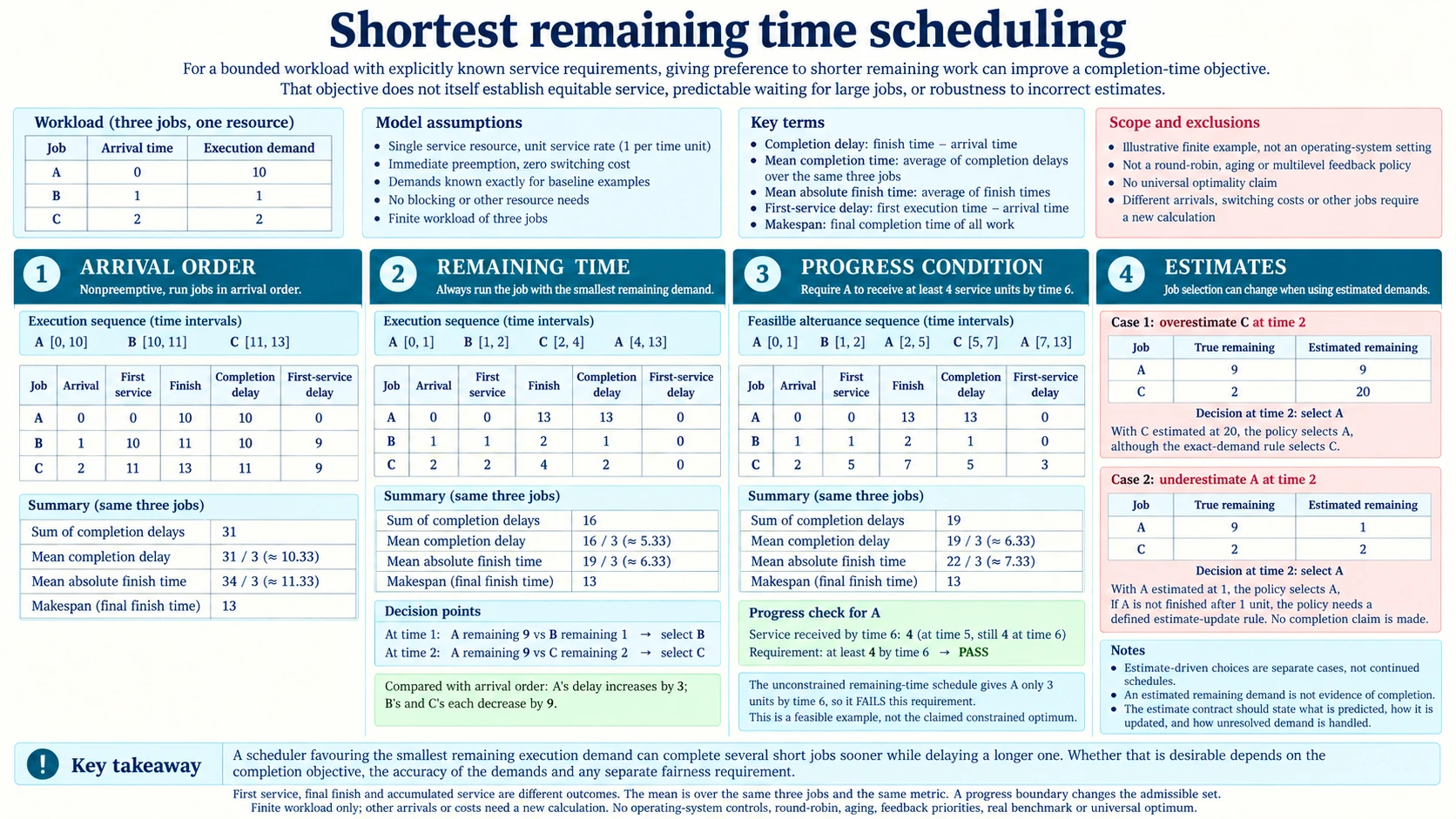
A scheduler favouring the smallest remaining execution demand can complete several short jobs sooner while delaying a longer one. Whether that is desirable depends on the completion objective, the accuracy of the demands and any separate fairness requirement. shortest remaining time scheduling therefore needs an explicit workload model. An improvement in the average for one finite example does not establish a universal policy for unknown sizes, switching costs or required progress guarantees. The examples use a single service resource and hypothetical time units. They are not operating-system settings, a round-robin quantum recommendation or measured application performance.

Define mean completion time and the workload

Let job A arrive at time zero and require ten execution-time units. B arrives at one and requires one. C arrives at two and requires two. Each receives service at one unit per time unit while executing. The model permits immediate preemption with zero switching cost. Demands are initially known exactly, and no job blocks or needs another resource. Ties would follow a stated stable rule, though the traced choices have different remaining demands.

Use arrival-to-finish delay as the mean completion objective. For each job, subtract its arrival time from its finish time, then average over the same three jobs.

Mean absolute finish time is another metric. For this fixed workload it differs by the constant mean arrival time, so the two orderings give the same preference when comparing their means. The report should still name which numbers it presents.

First-service delay is separate: subtract arrival from the time the job first receives execution. Starting promptly does not establish that the job finishes promptly.

The kernel-preemption guide supplies a dispatch-boundary comparison for mean completion time. Its urgent task H becomes eligible at one but first executes at nine, after a protected region ends at eight and a one-unit switch completes. That eight-unit delay ends at first execution; completion needs further work. Keeping those events separate prevents a first-dispatch observation from being used as a completion result. The three jobs below retain their own arrivals, demands and zero-cost preemption assumptions.

Calculate an arrival-order schedule

First use an arrival-order, nonpreemptive schedule under the same inputs. A runs from zero to ten, B from ten to eleven, and C from eleven to thirteen.

A finishes at ten with completion delay ten. B finishes at eleven, ten units after its arrival at one. C finishes at thirteen, eleven units after its arrival at two.

The mean completion delay is 31 divided by three, about ten and one-third. The mean absolute finish time is 34 divided by three, about eleven and one-third.

The first-service delays are zero for A, nine for B and nine for C. The long first job keeps the two shorter arrivals waiting even though they need relatively little execution.

The final completion time of the whole workload is thirteen. This makespan should not be confused with the mean of the individual delays.

Trace new short arrivals under the remaining-time rule

At zero, only A is present, so A receives one unit before B arrives. At time one, A has nine remaining while B needs one. The rule selects B.

B runs from one to two and finishes. C arrives at two with demand two, while A still has nine, so the rule selects C. After C runs until four, A receives its remaining nine units from four to thirteen. The whole workload still ends at thirteen.

The finish times are A at thirteen, B at two and C at four. Their completion delays are thirteen, one and two. The mean is sixteen divided by three, about five and one-third.

The mean absolute finish time is nineteen divided by three, about six and one-third. The average improved for this traced workload while A's completion delay increased from ten to thirteen.

Each job's first-service delay is zero in this history. A began immediately in both schedules but experienced a different later service pattern. Initial dispatch alone would hide the effect of the preemptions.

The average can improve while one job fares worse

Compared with arrival order, the remaining-time schedule reduces B's delay by nine and C's by nine, while increasing A's by three. The sum falls from 31 to sixteen. Those individual changes explain the lower mean and show exactly which job fares worse. They leave A's intermediate progress to be checked from its service intervals.

A policy can intentionally optimize the stated mean, but a caller caring about A's completion or service gaps has another objective. The average cannot settle that requirement by itself.

The same thirteen units of required execution appear in both traces. Their difference concerns which job waits and when, rather than a change in the amount of work. This is why the unchanged final finish time thirteen can coexist with a substantially different mean delay.

This article does not claim optimality beyond a specified scheduling model. The two histories demonstrate a concrete tradeoff without supplying a theorem for every real workload.

How job size estimation changes the selected order

Now replace exact demands with estimates used for selection. At time two, suppose A's remaining nine units are estimated correctly but C's true two units are estimated as twenty.

The estimated remaining-time comparison selects A rather than C. The earlier exact-demand trace no longer predicts the next execution choice. The estimate does not establish actual demand; C still requires two units under the supplied workload.

Another estimation error can underestimate A. If the policy believes A has only one unit remaining while C needs two, it can again prefer A. If A does not finish after that one unit, the policy needs a defined estimate-update rule.

The CPU-capacity guide provides a changed-profile example for job size estimation. Its task A has fifty work units at rate four followed by fifty at rate two, requiring 37.5 execution-time units instead of the constant-rate prediction of twenty-five. That changed profile misses a thirty-unit completion requirement. The guide converts work through task-specific service rates; our selection examples use remaining execution demand directly. Both calculations need an estimate that covers the remaining work, and neither prediction proves the task has finished.

The estimate contract should say what is predicted, how new evidence changes it, and how unresolved demand is handled. Treating an exhausted estimate as proof of job completion would misreport actual work.

No single observed short run establishes that future jobs have the same remaining demand. The scheduling objective and the evidence for its inputs remain distinct.

Add a progress requirement for the long job

Introduce a fairness constraint: by time six, A must have received at least four execution units. Keep the original exact demands and zero switching cost.

In the unconstrained remaining-time trace, A receives one unit before time one and two more from four to six. Its total at six is three, so that schedule fails the added requirement.

One admissible alternative runs A from zero to one, B from one to two, A from two to five, C from five to seven, and A from seven to thirteen. A has received four units by five, meeting the six-time boundary. B still finishes at two, C now finishes at seven, and A finishes at thirteen.

The completion delays become thirteen, one and five, giving nineteen divided by three, about six and one-third. The example's average is worse than the unconstrained trace, but the explicit progress rule is satisfied.

This alternative demonstrates feasibility under the progress condition; finding the best constrained schedule would require comparing the full admissible set. The constraint changes the set of admissible schedules before their means can be compared.

Specify which fairness property is actually required

The four-units-by-six requirement is an intermediate progress condition. It does not say that A must finish earlier than thirteen or that every job receives equal execution time.

Another application can impose a maximum completion delay or another stated service condition. Those requirements are different constraints and need their own calculations.

A generic fair status cannot identify which property the schedule met. The record should preserve the numerical or logical condition and the service intervals that test it.

The example does not introduce waiting-based priority aging or behaviour-based feedback priorities. It directly states one admissibility constraint so its effect on the original objective can be inspected.

Continuing short arrivals can present another progress question for a long job. A claim about an unbounded arrival stream would require assumptions beyond the three-job finite history analysed here.

Keep the outcome metrics and inputs separate

For each schedule, retain arrival, first service, accumulated service, finish and remaining demand. Compute the chosen mean over the same included job population.

A result comparing one job set's mean with another's would not establish the policy effect isolated here. Neither would switching from arrival-to-finish delay to absolute finish time without identifying the metric.

Keep estimate-driven choices separate from the exact-demand trace. An execution order based on C's estimated twenty cannot inherit the result calculated for known demand two.

Then test any fairness or completion requirements directly. A lower unconstrained mean cannot override a condition that defines which schedules the application accepts.

Verify the finite histories before making a policy claim

The arrival-order history must account for A ten, B one and C two service units, ending at thirteen. The remaining-time history must account for the same demand with the stated preemptions.

The average-delay comparison is 31 over three versus sixteen over three. The fairness alternative has nineteen over three and A's required four units before six. A passing check needs both the metric and the constraint evidence.

For the three-job delay worksheet, use the Lenovo IdeaPad 15.6-inch FHD touch laptop. For the saved history files, the catalogue identifies 512GB PCIe SSD storage; its processor and memory entries give i5-1334U and 16GB DDR4. Keep arrival, first service and final finish in separate columns. The A row then records first service zero in both histories but finish ten versus thirteen. Equipment identity can accompany the worksheet, while the stipulated intervals supply its scheduling evidence.

A second table on the ASUS Vivobook 14 FHD laptop can audit A's four-units-by-six requirement separately from the averages. The native description identifies the Core 5 120U processor and 16GB DDR4 memory. Enter A's accumulated service at six as three for the unconstrained history and four for the admissible alternative. That comparison tests a declared progress boundary; no real scheduler benchmark or hardware fairness guarantee follows from the catalogue entry.