How heterogeneous CPU scheduling compares work, time and energy

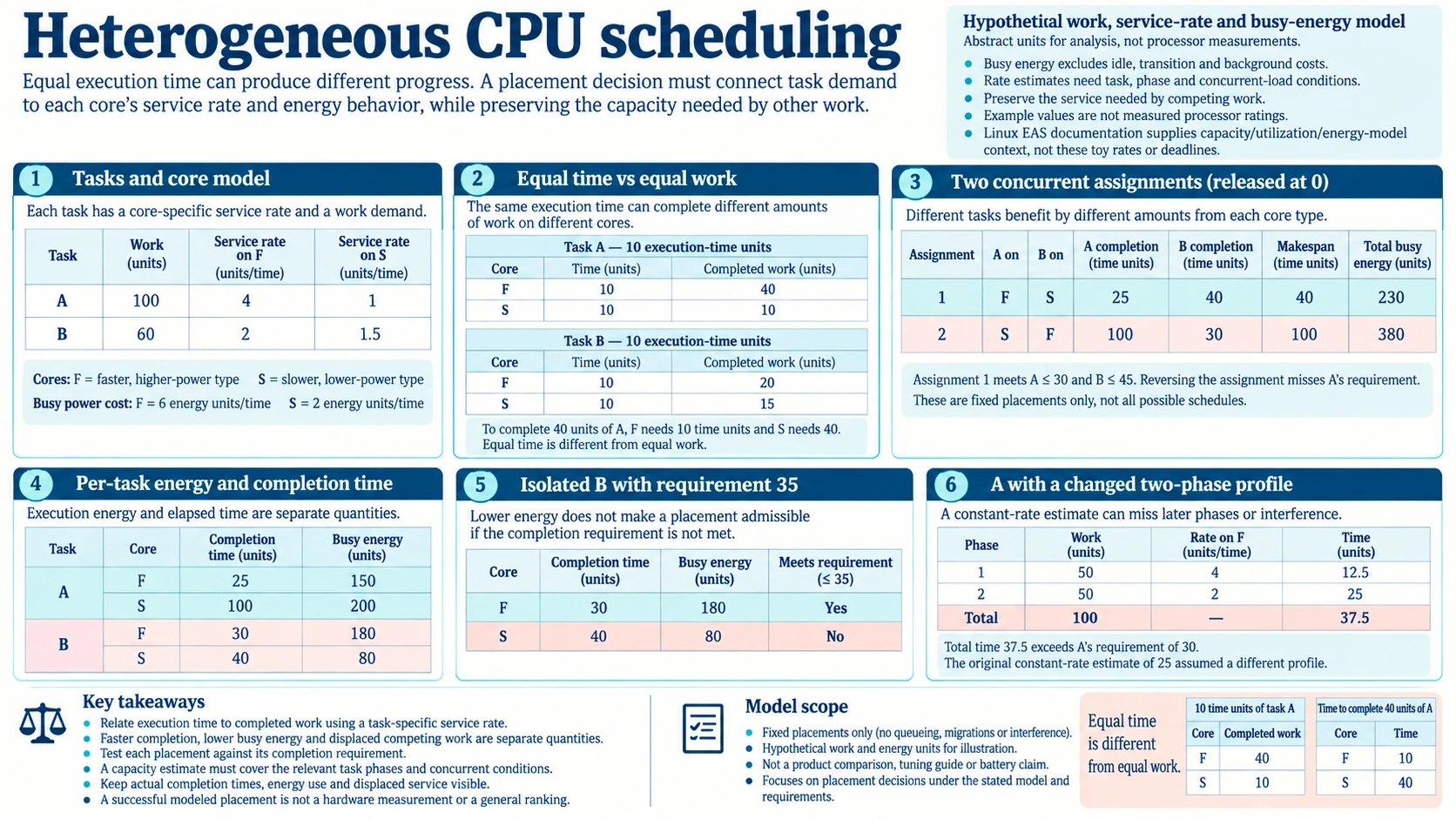
Equal execution time on two cores need not produce equal progress on a task. If the cores provide different task-specific service rates, a scheduling policy must relate time to completed work before comparing placements.

heterogeneous CPU scheduling uses that relationship under its stated capacity model. Faster completion, lower busy-energy cost and the service displaced from another task are separate quantities.

The examples define abstract work and energy units. They are not processor rankings, tuning instructions or measurements of a particular device's energy consumption.

Define core capacity through task-specific service

Use two core types F and S. For task A, stipulate a service rate of four work units per execution-time unit on F and one on S. A needs one hundred work units.

For task B, stipulate two work units per execution-time unit on F and one and a half on S. B needs sixty units. These rates are constant during the modelled execution and already describe the particular task.

Each task uses one core at a time in the placement examples. Tasks and inputs are initially ready, and the fixed-assignment calculations contain no queueing, migration or additional shared-resource interference.

F is four times as fast as S for A under these assumptions, but only four-thirds as fast for B. A single label saying F has four times the capacity would not predict both tasks correctly.

The work units belong to the defined task progress model. An execution-time counter does not establish them without a rate relationship, and a core's name alone does not supply that relationship.

The copy-on-write guide supplies a measurement-account comparison for core capacity. Its logical mapped size can stay unchanged while unique physical payload grows as pages become private. The exact quantity and sharing conditions determine what the counter means. Our execution-time counter likewise needs a task-specific rate before it can determine completed work. The page guide explains a different memory account; it supplies no CPU service rate or placement policy.

Equal time and equal work lead to different accounts

Give A ten execution-time units on F. It completes forty work units. Ten units on S complete ten. The time allocations match while the completed work differs.

To complete forty A units, F needs ten time units and S needs forty. Equal work therefore requires unequal execution time under this model.

For B, ten time units on F produce twenty work units, while ten on S produce fifteen. B's placement difference is smaller than A's even though the same cores and time interval are used.

A policy comparing execution times must state what fairness or completion objective those times represent. Equal time can be an intended allocation rule, but it is not automatically equal task progress.

This example concerns unequal service on different core types. It does not derive affinity restrictions for otherwise equivalent cores or an operating-system fairness quota.

Compare concurrent assignments with different relative benefits

Assign A to F and B to S at time zero. A completes its one hundred units in twenty-five time units. B completes sixty at rate one and a half in forty. The last of the two tasks therefore finishes at forty under this fixed assignment. Both can execute concurrently on their assigned cores, with no additional interference in the model.

Now assign A to S and B to F. A needs one hundred time units, while B needs thirty. The last completion is at one hundred. A's larger relative service benefit explains the first assignment's advantage. Giving F to B saves B ten execution units compared with S, while taking F away from A adds seventy-five.

This compares two specified assignments, not every possible schedule with migration or changing rates. An optimality claim over a broader scheduling space would need that space and its assumptions defined.

The displaced work matters even if one placement makes a single task faster. A local improvement for B can coexist with much later completion for A and the pair.

Account for execution energy separately

Stipulate busy power costs of six energy units per execution-time unit on F and two on S. These are teaching values. Idle energy, transition costs and whole-system background power are outside this numerical account.

A on F uses twenty-five times six, or 150 busy-energy units. A on S uses one hundred times two, or 200. The higher-power core completes A sufficiently faster to use less busy energy in this model.

B on F uses thirty times six, or 180 units. B on S uses forty times two, or eighty. For B, the lower-power placement uses less busy energy but completes ten time units later.

The first concurrent assignment totals 230 busy-energy units and finishes the pair at forty. The second totals 380 and finishes at one hundred. Those results follow from the stipulated task rates and power costs.

Execution energy is not synonymous with elapsed time or total device energy. A system can incur other costs while a task waits or after another task finishes. The toy totals cannot be converted into a laptop battery-life claim.

The analysis also does not assume every task is more energy-efficient on the same core. A and B already show different energy preferences under one pair of busy-power assumptions.

How energy-aware placement meets the completion contract

Give A a completion requirement of thirty time units and B a requirement of forty-five, both measured from the common release at zero. The A-on-F/B-on-S assignment meets both under the stated model. The reversed assignment completes B by thirty but leaves A unfinished until one hundred. B's individual improvement does not make that placement admissible for the two-task requirement.

The pipeline backpressure guide adds a whole-resource-account comparison for energy-aware placement. A queue-slot limit leaves running work and retained outputs outside that one boundary, so the pipeline needs its full resource ledger. Our placement assessment likewise retains both A and B, their completion requirements and the service displaced by assigning F elsewhere. The pipeline model bounds retained memory; the CPU rates, busy-energy costs and deadline checks here require their own stated assumptions.

Linux's Energy Aware Scheduling documentation describes using CPU capacity, utilization signals and an Energy Model when choosing a wake-up placement. Its energy estimate considers the relevant performance domains: raising one domain's operating point can increase the cost of tasks already running there. This gives a concrete implementation context for keeping competing work in the account. Its platform and utilization assumptions do not make our A/B rates measured processor values or establish the hypothetical completion deadlines.

For an isolated B with a requirement of thirty-five, S's forty-unit completion fails even though its busy energy is lower. F's thirty-unit completion meets that requirement at the higher model energy cost.

The policy chooses among the alternatives admitted by its actual constraints. Always selecting the lower-power type would fail the isolated-B example and would not even minimize A's busy energy.

Changing the requirement changes the decision problem. A placement's validity is not a permanent property of the core independent of the task and deadline.

A capacity estimate can miss phases and interference

The model used one constant rate for each task-core pair. A real progress estimate needs evidence that its work unit and rate cover the relevant execution, rather than only one favourable phase.

For an explicit changed profile, let A's first fifty units run at F's rate four, but its next fifty at rate two. The two service times are twelve and a half and twenty-five, totalling thirty-seven and a half. Reusing the constant-rate prediction twenty-five would incorrectly accept A's thirty-unit requirement. This counterexample changes the rate assumption, not the original arithmetic; it illustrates what the estimate must cover.

If A's later phase has another rate, the first twenty-five-unit calculation no longer describes the whole task. The scheduler must account for the changed remaining work and service assumptions.

Concurrent execution can also introduce resource interactions absent from the fixed-rate example. A measured solo rate does not independently establish the same service while another task runs.

The placement estimate therefore needs its observation conditions and uncertainty. A scalar capacity rating can be useful to a policy while remaining insufficient to predict every task's actual progress.

The limitations concern the declared service model. A hardware cause for an observed rate difference would require separate evidence beyond this placement calculation.

Keep elapsed time and displaced service visible

For a task that waits before execution, elapsed completion includes that waiting as well as service time. A placement calculation based only on work divided by rate omits the interval before the core actually runs it. If a task is preempted or another operation uses its intended core, the available service intervals also differ from the continuous execution assumed in the table. The result needs those intervals, not merely a nominal core choice.

For the concurrent pair, record both completion times rather than only the makespan. The first assignment gives A twenty-five and B forty; the second gives A one hundred and B thirty.

The energy comparison needs both per-task busy costs as well. A pair-level total can hide which task consumes more and why a tighter requirement changes the feasible choice.

A useful report therefore preserves work, task-specific rate, actual service, completion requirement and the work displaced by assigning the faster resource elsewhere.

Test the declared placement instead of ranking hardware names

Reproduce each task's service calculation under the stipulated rate. Check the completion requirement before comparing model energy among allowed alternatives.

The equal-time example must report forty versus ten A work units, not equivalent progress. The concurrent reverse assignment must retain A's missed thirty-unit requirement even though B finishes earlier.

For a real policy claim, identify the evidence supporting the rate estimates and any omitted waiting or interference. A successful modeled placement is not an implementation measurement.

Save work completed, actual execution time and busy energy as separate fields on the Lenovo IdeaPad laptop with a touchscreen, whose listing specifies a 15.6-inch FHD display. For the timing worksheet, its entry identifies 512GB PCIe SSD storage, along with an i5-1334U processor and 16GB DDR4 memory. Keep A's ten-time-unit outcomes forty and ten beside their F/S rates. The worksheet demonstrates the declared progress account, without treating catalogue hardware as its measured rate source.

Place the B deadline check beside its energy alternatives on the ASUS Vivobook 14 FHD laptop. The catalogue identifies 16GB DDR4 memory and a Core 5 120U processor. Record B's model completions thirty and forty beside busy-energy costs 180 and eighty. With a thirty-five-unit requirement, the lower-energy S alternative fails admission. That table establishes a hypothetical choice, not an energy optimum for the listed device.