Pairwise independence limits: three bits, one rule

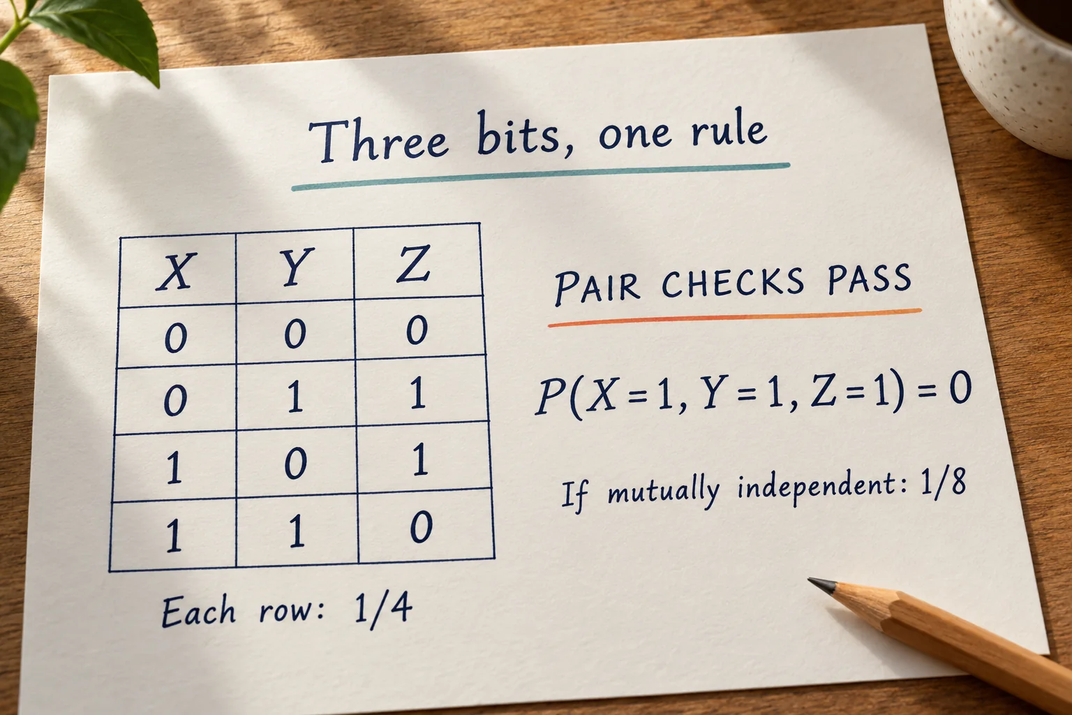
Pairwise independence limits become visible in a small probability model with only four possible records. Each record contains three bits, X, Y and Z. Every pair passes an exact independence check, yet the three variables are not mutually independent. Mutual independence requires a factorization of the full joint distribution.

The records and their weights are stipulated for this exercise. They are not observations from a device, a coin trial or a real dataset. That distinction matters: four observed rows would not establish that a real process assigns them the probabilities used here. Our task is to inspect a completely defined mathematical model and test a proposed inference from pairwise results to a three-variable conclusion.

Define the four equally likely records

Call the records A, B, C and D. Their X-Y-Z values are A: 0-0-0, B: 0-1-1, C: 1-0-1 and D: 1-1-0. Assign each complete record probability one quarter. No other three-bit record has positive probability in this model. The four weights add to one, so the listed records define the full probability distribution rather than a partial report about a larger unknown collection.

The third bit follows a fixed rule: Z is zero when X and Y agree, and one when they differ. This is the exclusive-or, or XOR, rule. For X = 0 and Y = 0, Z is zero; for 0 and 1, Z is one; for 1 and 0, Z is one; and for 1 and 1, Z returns to zero. The rule describes these stipulated bits, without establishing anything about a physical circuit or software implementation.

Keep each record's probability beside its complete triple. Merely writing four rows would not make them equally likely. Here equal weights are part of the definition, which makes the subsequent counts usable as exact probabilities. If someone changes a weight or introduces another record, that creates a different model requiring new marginal and joint calculations.

Check the single-variable probabilities

X is zero in A and B, and one in C and D. Each group contains two records of weight one quarter, giving probability one half for each value. Y is zero in A and C, and one in B and D, again giving halves. Z is zero in A and D, and one in B and C, so its two values also each have probability one half.

Thus every variable has a fair binary marginal distribution. The word “marginal” refers to looking at one variable while summing over the others. It does not say the variables are independent. Three separate half-and-half results leave open how the columns fit together in complete records. Retain the row identities so that a later pair or triple question can return to the full distribution.

Inspect all three pair tables

For X and Y, the four ordered pairs 00, 01, 10 and 11 appear respectively in A, B, C and D. Each therefore has probability one quarter. This equals one half times one half, the product of the corresponding single-variable probabilities. The full X-Y pair table factors as required for independence; the check covers every possible binary value assignment for that pair.

For X and Z, the records give A: 00, B: 01, C: 11 and D: 10. The order of the middle entries has changed, but each possible ordered pair still appears once. Every entry again has probability one quarter, equal to the product of the two relevant halves. X and Z are independent too. A different arrangement of row identities does not change those pair probabilities.

For Y and Z, the records give A: 00, B: 11, C: 01 and D: 10. All four ordered pairs occur exactly once, each with probability one quarter. Their entries also factor into the single-variable probabilities. We have now checked X-Y, X-Z and Y-Z. This is pairwise independence of the three variables, not a finding based on inspecting only one favored pair.

For these binary variables, the complete pair tables settle the pairwise question. Events such as a variable taking either permitted value or taking neither are then covered by summing entries or using total probability. We are not checking just whether two chosen events happen to have equal probabilities. The full value-by-value factorization is what makes the pair statements independent-variable statements.

Ask a genuinely three-variable question

Mutual independence would require the joint probabilities to factor across all three variables as well. For the assignment X = 1, Y = 1, Z = 1, the product of the single probabilities is one half times one half times one half, or one eighth. But 111 is absent from the defined sample space. Its actual probability in this model is zero, which differs from one eighth.

One failing assignment is enough to refute mutual independence. The pair results remain correct. The unsupported step would be treating those three successful pair checks as if they guaranteed every three-way factorization. The missing 111 record makes the distinction explicit without changing any of the original weights or replacing the definition of independence midway through the calculation.

The all-zero assignment supplies another check. Record A gives 000 probability one quarter, while the product of the three single zero probabilities is one eighth. This time the joint probability is larger than the product. The model therefore has both missing triples and triples with more weight than the mutually independent fair-bit model would assign. Neither pattern contradicts the uniform pair tables already verified.

Condition on one bit, then on two

Given X = 1, only C and D remain. Their original weights are equal, and their Z values are one and zero. Thus Z is still zero with conditional probability one half. Given Y = 1 instead, the surviving records are B and D, again splitting Z evenly. Learning either one of these bits alone leaves the other tested bit's marginal unchanged, consistent with the corresponding pairwise independence.

Now give both conditions X = 1 and Y = 1. Only record D remains, and it has Z = 0. Consequently the conditional probability of Z = 0 given both conditions is one. The conditioning event has probability one quarter, so this conditional probability is defined. The two pieces of information together determine what neither piece determined alone.

This is a probability statement about the stipulated records. It does not establish that one variable physically causes another or that someone changed a bit after observing a result. The XOR relation was part of the full model from the beginning. Conditioning selects records satisfying the stated information; it does not rewrite their original values or weights.

Separate overlap from dependence

Events can overlap and still be independent. In this model, X = 0 and Y = 0 overlap in A, with probability one quarter. That equals the product of their two probabilities, one half times one half. Their overlap therefore supplies an example consistent with independence, rather than an automatic reason to reject it.

Likewise, pairwise independence does not mean the four records must have no repeated bit patterns or that every complete triple must be present. The relevant pair tables already show exactly what the property requires. The three-way test uses a larger set of assignments. Keeping the tested variables and the event beside each probability prevents a statement about one pair from silently becoming a statement about the full triple.

Compare a second model with the same pairs

For a separate control, assign probability one eighth to every binary triple: 000, 001, 010, 011, 100, 101, 110 and 111. This is a different distribution. Each individual variable is again zero in four records and one in four, giving halves. For any chosen pair, each of its four value assignments appears in two records, giving probability two eighths, or one quarter.

The control therefore has the same single-variable distributions and the same three pair tables as the original four-row model. Its full joint table differs: 111 has probability one eighth, and 000 also has probability one eighth. Every triple entry equals the product of its three single probabilities, so the control is mutually independent. The original XOR restriction does not apply to this second model.

These two defined distributions show why pair tables alone cannot identify the full joint law. They agree on every pair entry but disagree on three-variable events. If a claim concerns all three variables, request the relevant joint information or a justified assumption that supplies it. Successful pair checks can be reported accurately without promoting them to a conclusion they do not establish.

Keep the supporting references separate

The clear wall file holder account shows one complete transparent single-pocket holder with integral mounting structure. Its native six-pack wording is not independently counted by that photograph. No maker identity, acrylic composition, dimensions, paper fit, load or mounting performance is authenticated here. It is optional paper-record storage context.

The four-pocket wire file and magazine holder account shows modular pockets with hanging loops and tag holders. Pictured documents, magazines and folders are unconfirmed supplies; the native blank tag papers are labeling supplies. Catalog Cosrack and description X-cosrack establish no maker equivalence here. No material, size, load, stability or mounting result is verified.

The repeated label puzzle counts an any-repeat event under an expressly fully independent six-symbol model, distinguishing that event from a mean matching-pair count. Here the question is whether independence of every pair implies mutual independence of three variables. No collision probability or pair-count average supplies the missing three-way factorization.

The five-mark stop game assumes independent half-and-half directions and examines endpoint chances and mean duration. Its stopped paths are a different model from the four static bit records here. An assumption that supports that walk's equations does not establish mutual independence for this separate joint distribution.

Keep a storage order outside the model

If a reader considers a separate organizer order, keep the item evidence apart from the probability worksheet. A uniform pair table establishes no supplied quantity, material, mounting fit or safe load. Before ordering through republeq.com, identify the exact listing, intended quantity and condition, and resolve any product question that affects the purchase. Documents or magazines pictured inside a holder do not automatically belong to its supplied contents. If cryptocurrency is being considered, inspect the payment choices actually presented for that particular order before choosing how to proceed. A guide mentioning USDT does not establish support for the token, a particular network or a particular wallet. Where a suitable cryptocurrency option is actually offered, verify the requested asset, network, destination, amount and order reference against the current instructions before authorizing a transfer. Include shipping, taxes and any transaction charges when checking the complete amount. Keep the item reference, applicable delivery and return terms, and any written clarification with the order record. If the item, quantity or payment instructions change, review the new information rather than treating an earlier answer as automatically current. Save the resulting order confirmation and payment record together so that a later inquiry can identify the specific transaction. An uncertain payment or order status calls for reconciliation against those existing records before considering another payment. None of those steps changes the four stipulated records or their equal weights. The mathematical counterexample can be checked without buying either optional storage item, while a later purchase depends on its own actual product and transaction information.