Anemometer airflow units: speed needs an opening area

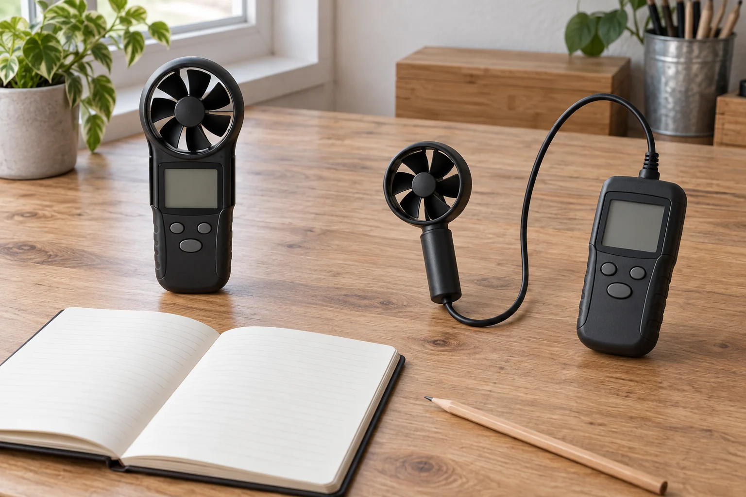
Anemometer airflow units distinguish the speed of moving air from the amount passing through an opening. A display marked metres per second answers a different question from one marked cubic metres per minute. An instrument can offer both kinds of figure, but a speed number alone leaves the opening's area unspecified.

The Unbranded KE-856A and LuckyBliss 416 offers both describe air-speed instruments with volume-flow functions. Understanding the quantities helps you read those claims before choosing equipment. This explanation uses invented openings and supplied fictional readings to develop the physical relationship. It gives no procedure for measuring a real duct, balancing ventilation or deciding whether a workplace or room is adequately ventilated.

Give air speed and volume flow different meanings

OSHA's Technical Manual defines an anemometer as an instrument measuring air velocity and describes area as the cross-section through which air moves. It distinguishes velocity from volume flow rate and explains that velocity can vary across a duct, making a single reading insufficient. Its glossary relates slot velocity to total volume flow divided by slot area.

For the simplified models here, the moving air travels straight through the opening, perpendicular to its face. The stated speed represents that direction and is uniform across the first opening. With those assumptions, air speed and volume flow connect through a geometric picture: imagine the air passing through as an invisible rectangular block.

Suppose the fictional opening is half a metre wide and four-tenths of a metre high. Multiplying those two lengths gives an area of 0.20 square metres. That area describes a flat cross-section. It is neither a length of travel nor a quantity of air by itself.

Now let the uniform air speed be three metres per second. In one second, the imagined block extends three metres along the direction of travel. Its base is the opening's 0.20-square-metre cross-section. Multiplying that base by the three-metre length gives 0.60 cubic metres passing through during that second.

The resulting rate is 0.60 cubic metres per second. The length unit from movement combines with the two length units in area, producing a cubic unit. That physical picture explains why an opening's dimensions matter. A speed display has supplied the imagined block's length per second; it has not supplied the size of its base.

Change the opening while keeping the same speed

Keep the speed at three metres per second, but halve the fictional opening's height to 0.20 metres while retaining its half-metre width. Its area becomes 0.10 square metres. The imagined one-second block is still three metres long, but its base is half the previous size.

The volume passing through is therefore 0.30 cubic metres per second. Both examples have the same speed. Their volume rates differ because their cross-sections differ. Equal speed readings therefore need not represent equal volume flow through differently sized openings.

Reverse the comparison next. Suppose the smaller 0.10-square-metre opening has uniform speed of six metres per second. Its flow becomes 0.60 cubic metres per second, matching the larger opening's earlier rate. The faster movement through the smaller base produces the same modeled volume per second as the slower movement through the larger base.

Neither example ranks actual fans or openings. They describe particular supplied areas and uniform speeds. A real system might change its speed distribution when its geometry changes. Holding one input fixed in a worked model does not establish that changing a physical opening will leave that input unchanged.

Read CMM and CFM as volume-rate labels

Return to the first model's 0.60 cubic metres per second. If that rate stays constant for a minute, sixty seconds each contribute 0.60 cubic metres. Multiplication gives 36 cubic metres per minute. The same model can therefore be described as 0.60 cubic metres per second or 36 cubic metres per minute.

The numerical value changed with the time interval. Thirty-six does not describe air travelling thirty-six metres each second, and it is not evidence that the fictional movement accelerated. Preserve the full unit when recording the value. Removing cubic or removing per minute changes the meaning.

A rate also differs from an accumulated volume. If the first fictional flow remains at 36 cubic metres per minute for five minutes, the passing volume is 180 cubic metres. The opening has not become a 180-CMM opening: 180 describes the amount accumulated over five minutes, while 36 describes its constant rate per minute. Keep the observation duration beside any accumulated amount.

If the same fictional opening instead passes 0.60 cubic metres per second for thirty seconds and 0.30 for the next thirty, the two intervals contribute eighteen and nine cubic metres. Their combined volume is 27 cubic metres over the minute. That sequence differs from maintaining the first rate for the full minute. A maximum speed alone cannot describe the total volume in this changing-flow example.

CMM denotes cubic metres per minute, while CFM denotes cubic feet per minute. Both describe volume rate. A figure in feet per minute instead describes speed. The extra cubic part matters: feet per minute and cubic feet per minute cannot be interchanged because their numbers happen to be similar.

The KE-856A description lists five speed units: metres per second, kilometres per hour, feet per minute, knots and miles per hour. Those are alternative speed labels. Its separate CMM/CFM account concerns volume rate. Switching among speed units does not, by itself, provide an opening's area.

Keep the cross-sectional dimensions attached to the calculation

Imagine someone copies the first opening's width as 0.50 metres but enters its height as 40 metres, overlooking that the original note said 40 centimetres. Multiplying those mismatched entries produces 20 square metres instead of 0.20. At the same modeled speed, the calculated flow becomes one hundred times the intended value.

The error began in the dimensions, before any airflow multiplication. Writing both dimensions in compatible length units restores the intended rectangle. This is an example about the fictional calculation, with no assertion about a particular instrument's entry screens, accepted units or error messages.

A circular opening needs its own geometry. Take an invented diameter of 0.20 metres, giving a radius of 0.10 metres. Using 3.14 for pi, its area is 3.14 multiplied by 0.10 squared, or 0.0314 square metres. With uniform speed of three metres per second, the modeled flow is 0.0942 cubic metres per second.

Using the diameter as though it were the radius would produce an area four times larger. Doubling a radius doubles each of the two length factors in its square. The resulting flow error would come from the wrong circular area, even if the copied speed and multiplication were otherwise correct.

Equal area can also come from different rectangular shapes. An opening one metre wide and 0.20 metres high has the same 0.20-square-metre area as the original half-by-four-tenths rectangle. With the same assumed uniform perpendicular speed, both produce the same calculated volume rate. This equality belongs to the stated geometry-and-speed model; it does not predict that two real differently shaped ducts have matching resistance or speed distributions.

The rectangle and circle are separate invented examples. The actual offers do not establish whether a particular instrument accepts width and height, diameter or a precomputed area. Establish the applicable input convention from the instructions for the exact instrument before relying on any displayed volume figure.

Use a supplied airflow map to understand a spatial mean

The earlier examples deliberately assumed uniform speed. To examine uneven flow, imagine a fictional 0.20-square-metre opening divided into two equal-area regions. A supplied drawing assigns one region a perpendicular speed of one metre per second and the other five metres per second. These are invented values for the entire regions, rather than measurements taken here.

The slower region contributes 0.10 multiplied by one, or 0.10 cubic metres per second. The faster region contributes 0.10 multiplied by five, or 0.50 cubic metres per second. Adding those contributions gives 0.60 cubic metres per second through the full opening.

Because the two regions have equal areas, their speed average is three metres per second. Multiplying that average by the full 0.20-square-metre area gives the same 0.60 result. In this particular map, averaging the two speeds works because each describes an equal share of the opening.

Using only the faster region's five-metre-per-second value for the whole opening would instead produce one cubic metre per second. That calculation silently extends the fast region's behavior across the slower region as well. The difference concerns the part of the opening represented by the speed input.

Now change the supplied map: half the area has speed one, one quarter has speed three and the remaining quarter has speed five metres per second. The regional contributions are 0.10, 0.15 and 0.25 cubic metres per second. Their sum is 0.50, while the simple average of the three listed speeds would incorrectly suggest 0.60 when applied to the full area.

The half-area region has twice the area of either quarter-area region, so each listed speed cannot receive equal weight. This example explains the role of represented area. It supplies no actual traverse pattern, grid size, probe orientation, sampling location or correction method for real equipment.

Separate anemometer averaging modes across space and time

For anemometer averaging modes, ask what varies among the values being combined. The fictional regional map describes different parts of one opening. A sequence recorded at one fixed point over time would describe change there. Its average would not automatically represent the rest of the opening.

Likewise, a held maximum preserves a different quantity from a spatial mean. The KE-856A offer names maximum, minimum, two-thirds maximum, average and real-time modes. The LuckyBliss 416 description names multi-point and timed mean calculations, maximum/minimum display and a Hold function. Those are actual listed functions, with no operating sequence or undocumented averaging algorithm supplied here.

The Unbranded KE-856A offer, SKU sku-18741464626 and UPC 710456857188, describes a separate vane sensor and USB data storage. The LuckyBliss 416 offer identifies SKU sku-17710664935 and an ABS housing. The number 416 does not establish that it is another manufacturer's instrument or shares that manufacturer's manual.

The weather-station reading guide separates current readings, update intervals and forecast horizons. Its weather-display timing discussion provides no airflow cross-section. The rain-gauge measuring-tube guide explains why a narrow tube can display collected water in a taller column. That concerns rainfall depth and a calibrated scale. Here, the opening and the air’s travel per second describe a passing volume rate, with no rainfall scale involved.

Reading anemometer airflow units begins with the complete quantity. A speed needs its distance and time units; a volume rate needs its cubic unit and time interval. In the worked opening models, the cross-sectional area connects them. The actual instrument's instructions and measurement conditions must establish whether its inputs and displayed result represent the real airflow question being asked.