How abstract interpretation widening reaches a useful result when program states keep growing

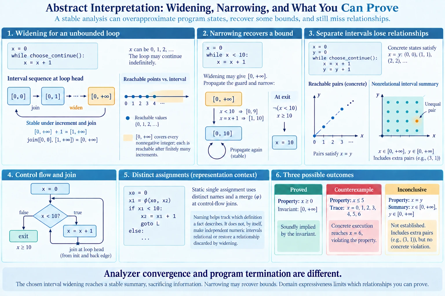
A loop can generate more possible values each time an analyzer follows its back edge. If the analyzer keeps every new value, its own computation can continue without reaching a stable answer. abstract interpretation widening addresses that problem by expanding a summary more aggressively than the program's next iteration requires. The resulting summary includes the states the analyzer needs to cover, while deliberately giving up some distinctions. That loss can leave a question unanswered even when the analysis finishes.

Consider a loop over mathematical integers. This assumption removes machine overflow from the example; a checker for a real language must use that language's arithmetic rules. We will first let a loop continue or stop nondeterministically, then add a bound. These small examples separate the program's behavior from the analyzer's behavior and make the discarded information visible.

Concrete states and sound approximation

x = 0
while choose_continue():
    x = x + 1

Here, choose_continue may return true or false on each visit. At the loop head, immediately before that choice, x can be 0, 1, 2, or any larger integer. A concrete state records an exact value at an exact program location. A concrete transition relates one state to another according to the next instruction. Starting from x equal to zero, the reachable states are those produced by taking any allowed finite sequence of transitions.

The reachable-state question concerns all those permitted executions. Tracing one execution that stops after three increments establishes that x equal to three is reachable. It says nothing about the executions that take four increments, or those that continue indefinitely. To reason about every permitted execution, an analyzer needs a representation that can cover many states at once.

An interval is one such representation. The interval [0, 5] includes every integer from zero through five. Its concretization is that set of integers. An interval summary is sound at a program point when its concretization includes every reachable concrete value at that point. It may also include values that no execution reaches. The interval [0, 5], for example, would safely summarize the set {0, 2, 5}, although it loses the holes between those values.

This is the direction of sound approximation used here: the analysis may include extra possibilities, but it must cover all actual possibilities allowed by its model. A summary that accidentally excludes x equal to five could support an incorrect safety claim. A wider summary can instead prevent a correct claim from being established. The difference matters when interpreting a warning.

Why ordinary fixed-point program analysis keeps growing

At the loop head, information arrives from the initialization and from the back edge. Joining intervals means taking an interval large enough to include both incoming intervals. The join of [0, 0] and [1, 1] is [0, 1]. Applying x = x + 1 to [0, 1] produces [1, 2], which joins with the initial value to produce [0, 2].

Repeating the calculation yields [0, 0], [0, 1], [0, 2], [0, 3], and so on. Each interval includes the preceding one. Each finite summary still has a finite upper bound, so the next calculation enlarges it. The exact reachable set has a compact interval representation, [0, +infinity], but this particular iteration does not arrive there in finitely many increments.

A fixed point is a summary that the analysis equations no longer change. A sound invariant can also be a post-fixed point: propagating its states through the relevant transitions and joining the initial states yields something contained in the summary already available. Such closure supports reasoning about arbitrarily many loop iterations without enumerating them.

fixed-point program analysis depends on the abstract domain and the propagation rules. A domain with finite height cannot contain an indefinitely ascending chain of distinct elements. With suitable monotone transfer functions and the usual iterative construction, that helps ensure convergence. The unrestricted integer interval domain admits the ascending chain above, so this simple iteration needs another convergence mechanism.

A verifier can also propagate summaries through instruction sequences. The planned bytecode verification guide examines sound approximation through abstract execution states used to check bytecode structure, including operand and local-type requirements. That is a different property from the growing numeric bounds in this example. The connection is the use of summarized states and control-flow joins; the rules being checked determine what information those states must retain.

An explicit interval widening rule

For intervals A = [a, b] and B = [c, d], use the following simple widening rule. Keep the old lower bound a if c is no smaller than a; otherwise replace the lower bound with negative infinity. Keep the old upper bound b if d is no larger than b; otherwise replace the upper bound with positive infinity. This operator includes both A and B. The infinity symbols describe unbounded intervals of mathematical integers.

Widen [0, 0] with the next candidate [0, 1]. The lower bound remains zero because it has not moved downward. The upper bound moves upward, so widening replaces it with positive infinity. The new summary is [0, +infinity]. Incrementing that interval produces [1, +infinity], and joining the initial zero produces [0, +infinity] again. The summary is closed under the loop calculation.

The analyzer has stopped distinguishing how large x could become after a particular finite number of increments. It has retained nonnegativity. That retained fact is useful: under the stated arithmetic and transition rules, x cannot be negative at the loop head. The analysis does not establish an upper bound, because the program itself has none at that location.

Widening choices influence other examples more strongly. An analyzer can delay widening, use selected thresholds, or apply different operators for another abstract domain. Those policies require their own convergence argument. The rule above is intentionally coarse so that the exact loss is easy to inspect; it is not a description of every production analyzer.

Narrowing can recover a bound without recovering histories

x = 0
while x < 10:
    x = x + 1

For this bounded loop, the reachable values at the loop head are zero through ten. Ordinary interval iteration can reach [0, 10] after enough updates. If the analyzer applies the simple widening rule early, it can instead obtain [0, +infinity], discarding an upper bound that the program does have.

Now propagate that widened summary through the actual condition. On the true branch, x < 10 restricts mathematical integer values to x at most nine. Combined with the retained lower bound, that branch gives [0, 9]. Incrementing gives [1, 10]. Joining the initialized zero gives [0, 10] at the head. The guard has supplied information that the earlier widening step discarded.

A simple interval narrowing policy can replace an infinite bound with the corresponding finite bound from this recomputation. In this case it refines [0, +infinity] to [0, 10]. Propagating again yields the same interval. On the exit branch, x is at least ten, so intersecting that condition with [0, 10] establishes x equal to ten.

This particular result is precise, but narrowing is not a promise to reconstruct everything widening lost. The refined state contains values, not a record of which iteration introduced each value. In more complicated programs, joins may have already merged branches or discarded relationships that this interval domain cannot express. A refinement policy also needs sound transfer rules and a suitable termination strategy. Arbitrarily intersecting a summary with a desired result would not supply either.

A reader can work through these interval updates in a small script or a written table. The Lenovo IdeaPad 15.6-inch FHD Touch laptop listing describes an Intel Core i5-1334U, 16GB DDR4, and a 512GB PCIe SSD. It is a possible computing workspace for such an exercise. Those listing specifications do not establish analyzer compatibility, execution speed, or the correctness of an interval implementation; the exercise's assumptions and update rules determine its reasoning.

Separate variable bounds lose relationships

x = 0
y = 0
while choose_continue():
    x = x + 1
    y = y + 1

At the loop head, every reachable pair satisfies x equal to y. The concrete pairs are (0, 0), (1, 1), (2, 2), and so on. A nonrelational interval summary records one interval for x and another for y. After widening, both can be [0, +infinity]. Interpreted together, those intervals include the pair (0, 7), even though no execution of the stipulated loop reaches that pair.

The summary still covers every reachable pair. It has lost the relationship between the variables. An assertion that x equals y cannot be proved from these independent intervals, because their represented state set includes unequal pairs. Tightening either variable's individual bounds would not, by itself, express equality across an unbounded sequence.

A relational domain can represent constraints involving more than one variable. A representation that retains x - y = 0 can preserve the equality when both assignments increase their respective values by one. Its transfer and convergence machinery must support that representation soundly. More expressive domains can incur additional computation, and their precision still depends on how the analyzer handles joins and widening.

Variable naming also affects how an analysis organizes its facts. For context on the variable representation used by fixed-point program analysis, the static single assignment guide explains distinct assignment names and the merging of definitions when control-flow paths meet. That representation helps identify which definition a fact concerns. It does not automatically make independent numeric intervals relational or restore a relationship discarded by widening. The distinction prevents a naming convention from being credited with a proof the abstract domain cannot express.

Proof, counterexample, and an inconclusive result

Suppose an assertion requires x to be nonnegative in the first loop. The invariant [0, +infinity] implies that property, so the analyzer can establish it within the stated model. To trust the conclusion for an implementation, the model must cover the implementation's behavior, including arithmetic and any relevant exceptional transitions.

Suppose instead the assertion requires x to remain at most five. The concrete execution that takes six increments reaches x equal to six and violates that assertion at the head. A trace with those allowed transitions is a counterexample. The widened interval's inclusion of six is consistent with the violation, but inclusion alone would not prove that six is reachable in every program producing the same summary.

The paired-variable example shows the third outcome. The separate intervals include (0, 7), so they cannot establish x equal to y. Yet the program's transitions preserve equality. Reporting that the property was not established is accurate. Reporting a confirmed violation from the interval pair alone would confuse an extra abstract possibility with a concrete execution.

For a workspace with a different listing, the ASUS Blue 14 FHD laptop is identified by that title on its product page. It provides another product reference for a reader considering where to write and inspect analysis examples. The page title supplies no measured analyzer result. Comparing proof outcomes requires keeping the program, domain, and convergence policy fixed, regardless of which computer displays the table.

When reading an analyzer result, ask which program states its summary includes, which distinctions its domain can express, and where the convergence policy enlarged that summary. Then examine the property itself. A closed overapproximation may imply the property, a concrete trace may refute it, or the available summary may leave it unresolved. The analyzer's termination and the analyzed program's termination remain separate questions: even the nondeterministic loop with a possible infinite execution has a stable widened summary.